Distance Matrix Analysis and Spatial, Non-Spatial and Temporal Querying with QGIS
Contents
Purpose
The objective of this tutorial is to demonstrate how to convert non-spatial data files such as CSV files into shapefiles, how to complete a Distance Matrix Analysis, and how to query spatially, non-spatially and by time using Quantum GIS 3.4.14. This tutorial will be done using open source data. This tutorial compares significant earthquakes from 1990 - 2013 in North America and their relation to Populated Places in the Americas. The earthquake data was retrieved from the Significant Earthquake Database on the National Oceanic and Atmospheric Administration Website [1], and the Populated Places data was retrieved from the Natural Earth Website [2]. Additionally, this tutorial will also make use of fire disturbance data to demonstrate how to query using time as a selector using Ontario GeoHub Data [3]
The Purpose of this tutorial is to fulfill the partial requirements of the GEOM 4008 - Advanced Topics in Geographic Information Systems class' final exam project at Carleton University. The purpose of this project was to explore the advantages and disadvantages of different open source geographic information systems (GIS) programs.
Introduction to Quantum GIS 3.4.14
Quantum GIS 3.4.14 is a free Open Source Geographic Information System (GIS) program that is used to create, edit, visualize, analyze and publish geospatial information. The program is available for Windows, Mac, Linux, and BSD. This user friendly Open Source GIS program is licensed under the GNU General Public License and is an official project of the Open Source Geospatial Foundation. [4]
QGIS has many different features including QGIS Desktop, where you can create, edit, visualize, analyze and publish geospatial information; QGIS Browser, where you can browse and preview your data and metadata as well as move around your stored data; QGIS Server, where you can publish your QGIS projects as OGC compatible WMS and WFS services; and QGIS Web Client, where you can publish your QGIS projects.[5]
Downloading QGIS
Before beginning the tutorial, if you do not have the 3.4.14 version or above of QGIS please follow the steps below:
- Follow this link to download [6]
- Choose which version is compatible with the computer you are working on
- Follow the steps in the pop-up downloading window
Acquiring the Data
To download the Earthquake data follow these steps:
- Visit the Significant Earthquake Database at this link [7]
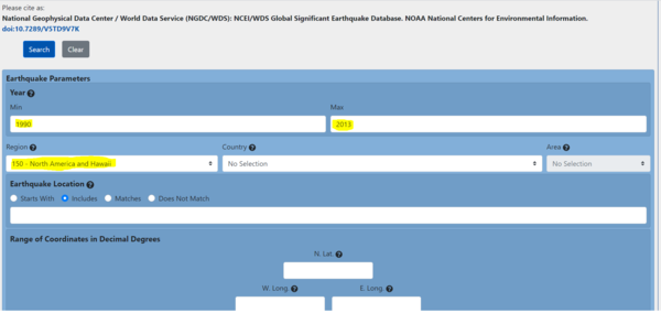
- Fill in the date of the form beginning by setting the minimum year to 1990 and the maximum year to 2013
- Select North America and Hawaii as the Region Name
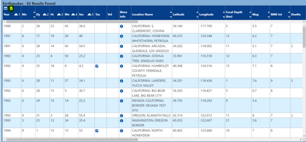
- After you pressed search and the data is presented, click the download .TSV button in the top left.
- Open up Microsoft Excel and open the .tsv file in Excel.
- The text import wizard will be activated and you must step through all the steps with the defaults.
- Your data will appear and then you must delete row 2 as it just contains information about your search query.
- Finally, save your file as a .csv file type.
To download the Populated Places data follow these steps:
- Visit the Natural Earth Website at this link [8]
- Click to download the Simplified (Less Columns) layer of the Populated Places.
- Download the file
- Unzip the file
- Save to same folder as the the Earthquake file
Tutorial
Adding Your CSV File
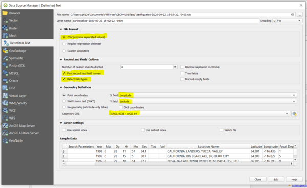
- Once QGIS opens, start by opening the Data Source Manager and clicking to Add Delimited Text Layer
- Fill in the Highlighted Forms Above with the proper information and attach the .csv file you created.
- Make sure you select WGS84 as your CRS.
DISCLAIMER: if an error occurs, it is because one of your features does not contain proper coordinates.
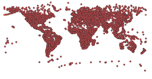
- Your CSV layer will now added to QGIS as you can see in your layer view.
Distance Matrix Analysis
A distance matrix analysis is a type of analysis performed when the user wants to know how far away certain things are from other things. In this case, we want to know how far away each earthquake is from the nearest city. After we have this matrix, we can perform a join that will merge our two tables together to give us an in-depth look at all of the data we have available to us.
- The first step we need to take is to add the Populated Places point file we downloaded earlier.
- Navigate to the Data Source Manager and and then navigate to the Vector tab.
- Navigate to where you stored your point file and enter it into the required field and click add.
- The layer should now look something like this:
- Now to begin the analysis by creating a distance matrix
- Using the Vector drop down menu on the tool bar, navigate to Analysis Tools and select Distance Matrix.
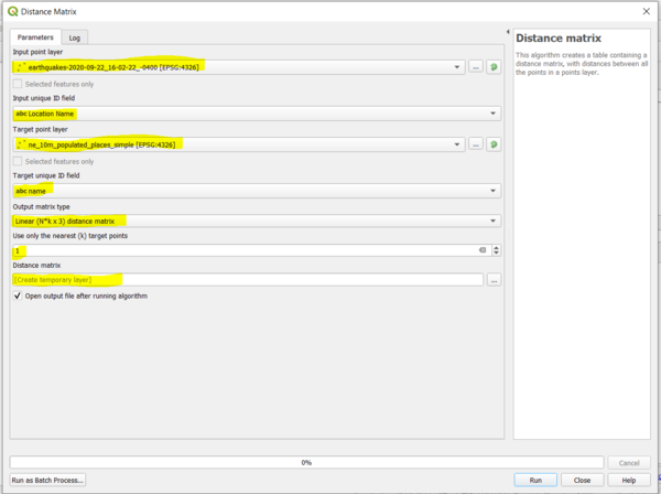
- To fill in the Distance Matrix Window, select Earthquakes as you Input point layer, Location Name as your Input Unique ID field, the Populated Places layer as your Target Point layer, and the Name of the Populated Place as the Target Unique ID field.
- The Output Matrix Type we are going to pick a Linear (N*k x 3) distance matrix and input 1 for the nearest target points. This is because we are looking for the nearest city to each earthquake and we want to dispose of the unnecessary data. Lastly, enter where you want this matrix file to be stored and ensure you add it to your data frame.
- An example of the parameters filled out is below:
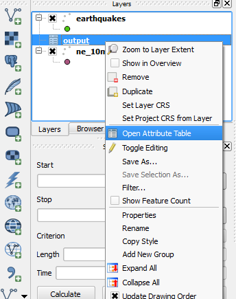
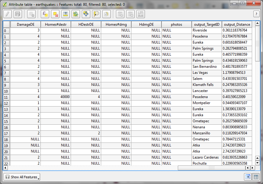
- To view the results of the Distance Matrix, RIGHT Click on the matrix in your Layers window on the left side of QGIS Desktop. Then click on Open Attribute Table, much as displayed in the image below:
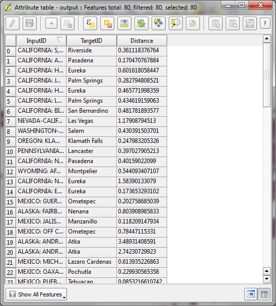
- The attribute table of the Distance Matrix should look similar to below, where the first column is the Name:Location of the earthquakes, the second column shows the closest populated city by Name to the earthquake. The third column is a distance in degrees and can be ignored as we are only looking for the closest cities to each earthquake.
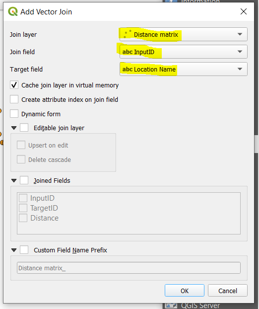
- To make our queries easier, we are going to join the matrix attribute table to the earthquake attribute table. To do this right click the earthquakes layer, and select properties. Navigate to the Joins tab and click the green plus button. Then use the distance matrix as the input file and the input ID as the Join Field. Finally, select name as your target field. The parameters for the Join and the expected output can be seen below. Congrats! You can now easily see which cities are closest to each of the earthquakes in our data set. Next we will learn about how derive information by analyzing the data with queries.
Querying
Querying is the process of using an expression to select a subset of features within a data set. It can be used to derive all sorts of different information for geoprocessing and other use cases. We will begin with the basics of how to query and then follow by three different examples.
- Open the attribute table of the joined earthquake data and click on the Select Features Using an Expression
First Example
The first example will run through how to use a query expression to determine that amount of earthquakes that occurred during the month of August.
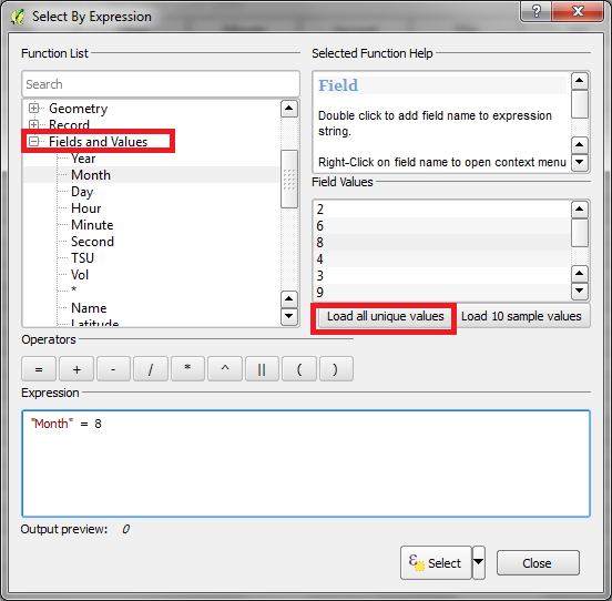
- Using the Select by Expression window selected in the Earthquakes Attribute table, under the Function List select the Fields and Values category and double click on Month.
- Now under the Operators list, select the equals (=) sign,
- Next, under the Field Values List select Load all Unique Values. This will load all the possible values under the Month Column.
- Double click on the 8(representing the 8th month of the year)value under Field Values or type the number into the Expression box.
- The expression should look identical to what appears in the image below:
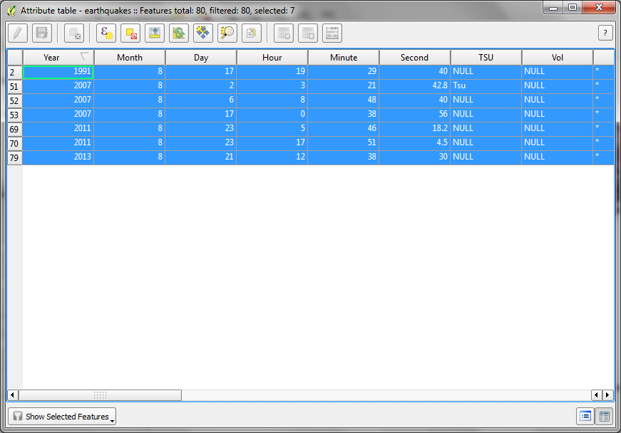
- Now looking at the attribute table, toggle to Show Selected Features at the bottom of the window and all the selected features will appear selected in the attribute table.
- The selected features in the image below, show that there were 7 of the 80 earthquakes occurred during the month of August.
Second Example
The second example will run through how to use a query expression to determine the amount of Populated Places with a population larger than 100,000.
- Using the Select by Expression window of the Populated Places layer's attribute table select the Fields and Values tab.
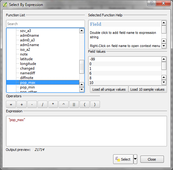
- Double click on the feature called pop_max
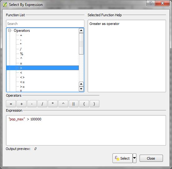
- Double clicking will add the category to the expression box, much like what is shown in the image below:
- Now under the Function list scroll up to the Operators tab.
- Select and double click the greater than symbol (>) under the operators tab, or manually type in the greater than symbol into the expression box.
- now manually type in 100000 into the expression box so the query expression looks like the expression in the image below:
- Click Select
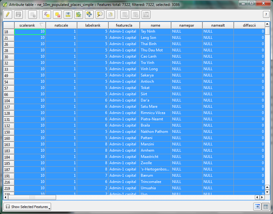
- The selected features will appear highlighted in your attribute table.
- The image below shows that there were 3086 out of the 7322 Populated Places that had a population larger than 100,000.
- To deselect the selected features click the Unselect All button on the Attribute table tool bar.
Third Example
The Third example will be to determine how many Populated Places Names begin with the letter F and end in the letter S.
- Follow the steps above, but this time under Fields and Values tab select Name.
- Double click Name so it appears in the expression box, then open the Operators tab.
- Select and double click LIKE
- Now in the expression box using single quotations type 'F%'. The % symbol represents a wildcard. This means that any number of combinations of letters behind the letter F is acceptable in the selection. The % symbol can be typed on manually or selected through the Operators tab.
- Now using the operators tab again select AND or type it in manually. This will allow two queries to be strung together.
- Now you can type this in manually with quotations around it or go back to the Field and Values tab and double clickName again.
- Now back to the operators tab or type in Manually LIKE
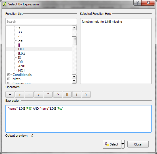
- After the LIKE now type in manually '%S'. Here we put the wildcard before the S because we want to select any number or combination of letters, only ending in S.
- The query expression should look like this:
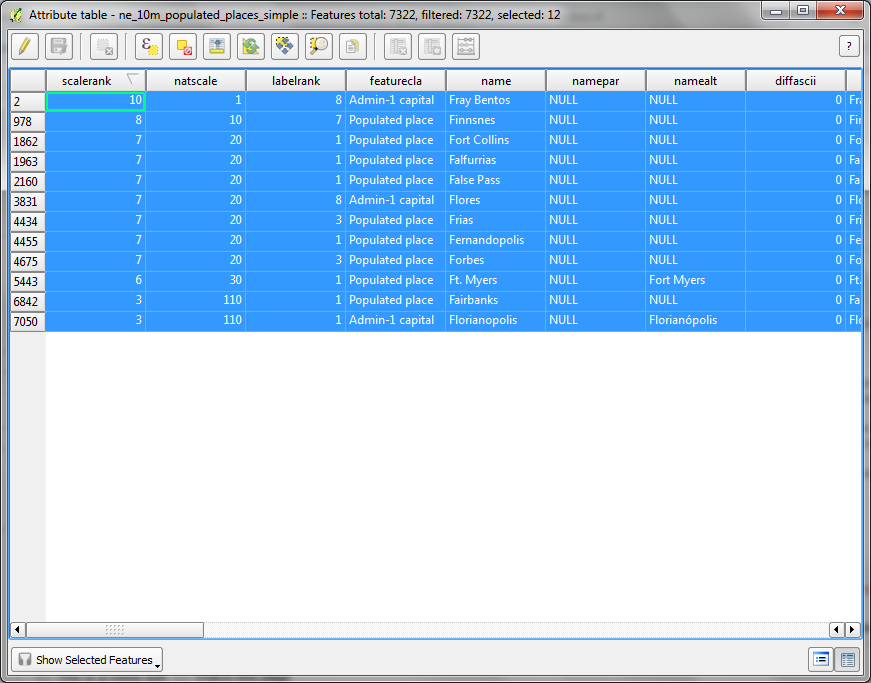
- After clicking Select the selected features will appear highlighted on your Attribute table.
- The following image shows that there were 12 out of the 7322 feature names that started with the letter F and ended in the letter S.
The next important aspect of querying is about how to spatially query and select features. We are going to combine what we learned in the previous examples to allow for queries that are spatially enabled. Results will not be precise as we are in a GCS, we will now project our layers into a projected coordinate system by clicking on the espg button on the bottom right of our dataframe. Enter the espg code 102008 and apply this pcs. The you will need to use the reproject tool on the earthquake data and the population data. This will allow us to create accurate buffers on the Western side of America.
- Begin by selecting the Vector tab in QGIS and then selecting Research Tools > Select by Location
- You can see on this page that many of same features in ESRI software are also available here. However, you will notice that we are missing the search by distance from or near.
Spatial Querying by Distance
- Ensure you have followed the above steps about reprojecting into a projected coordinate system (espg: 102008).
- In this example, we will look at which cities were within 100 km of an earthquake that happened in the 90's and had a magnitude of 7 or higher.
- The first step is to open the attribute table of the earthquakes and build the query
Year like '199%' and "Mag" >= 7 - Next, we will create a buffer of 100 km around our selected features.
- Navigate to Vector > Geoprocessing Tools > Buffer and open the buffer tool.
- Ensure the Selected Features Only tool is activated, enter a distance of 100 km, and put segments to 5 in order to produce a circle. This will create buffers for ONLY our desired features and allows us to now add a spatial component only to these desired layers.
- Navigate back to the select by location tool by going to Vector tab in QGIS and then selecting Research Tools > Select by Location
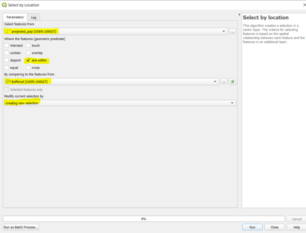
- Enter your population layer into the "Select features from" and your buffers into "By comparing to the features from". Then check the "within box". An example image is below:
- You will now see that that there are highlighted yellow cities that were contained within the buffers we made. Congrats! You have completed a near distance search in QGIS.
- In order to get these selected features into a new layer, you will need to right click on the population layer and press save selected features as.
- You can now even make even more sub-selections based on this spatial selection.
Spatial queries are the bread and butter of a GIS and allow the software to be extremely powerful. Many of the other spatial predicates that are found in other GIS software
are also available in the Select By Location tool.
Querying by Time
The last type of query we will cover is about how to easily query and display data using a time stamp. For this example, we will download a fire disturbance point file from Ontario's Geohub. It contains 50 thousand plus fire disturbances going back all the ways to the 1970's. It is a large amount of data to work with and it would be useful to know how to easily visualize it using the built in time stamps. We will be utilizing a really cool QGIS plugin to easily visualize the data.The plugin is called TimeManager. Start by downloading and extracting the data set from [[9]].
- Input the dataset into a freshly opened QGIS file.
- Go to Plugins > Manage and Install Plugins and when the popup appears, search for "TimeManager".
- Download the plugin, and it should appear on your toolbar above and should open automatically on the bottom of your data frame. If it does not appear automatically, right click your toolbar and make sure to tick the "Time Manager Panel".
- Click the settings in the time panel.
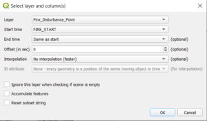
- Enter the "Fire Start" field as the date time, and the plugin will automatically detect if it is a valid date stamp. You can see what type of date stamps are valid in the description of the tool. Our example data has valid dates, but if this does not work on your data, this may be a reason why. There are also some useful options such as accumulating the new features with the features that had already been shown and by skipping over time slots that are empty. For this example, we will leave all the defaults.
- Click okay and you will now be back at your data frame view.
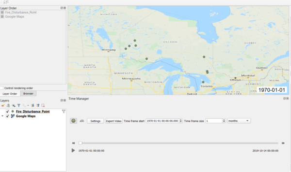
- We can now see our time slider, with our time stamp displayed on our map. Please note I have put in a basemap layer for context using the HCMGIS plugin.
There is a few key features of this panel that you must be aware of to effectively query by time.
- You can use the "Time Frame Start" to choose where the beginning of the slider is.
- You can use the time frame size and drop down menu next to it to dictate what type of time frame you want to see (ex. 1 year, 1 month, 1 day ect)
- Lastly, you can use the slider to find certain time periods, or you can choose a frame and let it play out over time to visualize the temporalspatial relationships.
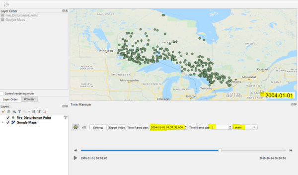
- In the next example, I will use this tool to query for all the fire disturbances that occurred throughout the whole year of 2004. Please note the highlighted areas. I have manually entered my time frame start which updates my data frame, and I have chosen a year as my frame with my starting time at the beginning of the year. This will display all the events that occurred that year.
This is the end of the querying by time portion of the tutorial. As you can probably see, this could be extremely useful for visualizing and querying for temporalspatial relationships and patterns. This tool can make it easy for you to see what is occurring where, how fast it is accumulating and even to create custom animations. It is by far one of the easiest ways to quickly query by varying amounts of time.
Querying Extras
For more information and example of different queries to run in QGIS visit the following links:
- For specific information on the QGIS Query Builder click here
- For other examples of how to build query expressions click here
- For an explanation of all the different operations click here
- For run through of querying using a YouTube tutorial click here
Resources
ArcGIS Resources (October 25, 2012). ArcGIS Help 10.1:Building a query Expression. Retrieved on December 17, 2013 from http://resources.arcgis.com/en/help/main/10.1/index.html#//00s50000002t000000
GeoInformation. (January 13, 2013). Tips and tutorials on working with GIS: Queries in QGIS. Retrieved on December 18, 2013 from http://infogeoblog.wordpress.com/2013/01/13/queries-in-qgis-pt-1-attribute-queries/
Harvard CGA (November 28, 2011). QGIS 5-Attribute Query [Video File] Retrieved on December 18, 2013 from http://www.youtube.com/watch?v=jRV6b_pd_PE
Natural Earth. (2013). Natural Earth: Populated Places. Retrieved November 19, 2013, from http://www.naturalearthdata.com/downloads/10m-cultural-vectors/10m-populated-places/.
NOAA. (November, 2013). The Significant Earthquake Database. Retrieved November 19, 2013, from http://www.ngdc.noaa.gov/nndc/struts/form?t=101650&s=1&d=1
QGIS. (2013) Download QGIS for your Platform. Retrieved on November 14, 2013 from http://www.qgis.org/en/site/forusers/download.html
QGIS. (2013). Features of QGIS. Retrieved on December 16, 2013 from http://www.qgis.org/en/site/about/features.html
QGIS. (December 15,2013). QGIS: A free and Open Source Geographic Information System. Retrieved December 16,2013, from http://www.qgis.org/en/site/index.html
QGIS. (2013). Query Builder. Retrieved on December 17, 2013 from http://www.qgis.org/en/docs/user_manual/working_with_vector/query_builder.html

