Hydrological & Terrain Analysis using WhiteboxTools

Introduction

WhiteboxTools is an open source geospatial analysis engine that includes more than 475 tools covering terrain and hydrological modelling, geospatial data analysis, remote sensing, imagine processing, LiDAR handling and general GIS workflows. Many of these tools go beyond the standard functions available in QGIS which makes it useful for complex and specialized spatial analysis. Since QGIS can call WhiteboxTools directly through the Processing Toolbox, the two systems integrate smoothly and allow for powerful and flexible analysis within one environment.

Purpose of Tutorial

This tutorial walks through the process of using WhiteboxTools inside QGIS to perform a complete hydrological and terrain workflow. The goal is to show how to take a raw DEM and turn it into a fully visualized Topographic Wetness Index, explaining how each step fits into the overall analysis in the process.

The steps covered include:

• Preparing and correcting a DFEM
• Generating flow direction and flow accumulation
• Deriving slope
• Calculating the Topographic Wetness Index (TWI)
• Improving visualization with symbology and optional hillshade

By the end, you should have both a working TWI raster and a clear understanding of how each WhiteboxTools step contributes to the final result.

Data & Software Requirements

• 30 m DEM of the Kananaskis region
• QGIS
• WhiteboxTools Open Core

Installing WhiteboxTools

Downloading WhiteboxTools

To download WhiteboxTools, head to the WhiteboxTools Download Page and download the WhiteboxTools Open Core. After downloading, extract the .zip file and place the folder somewhere easy to find. For example, you may store it in: C:\Program Files\WhiteboxTools\

Configuring WhiteboxTools in QGIS

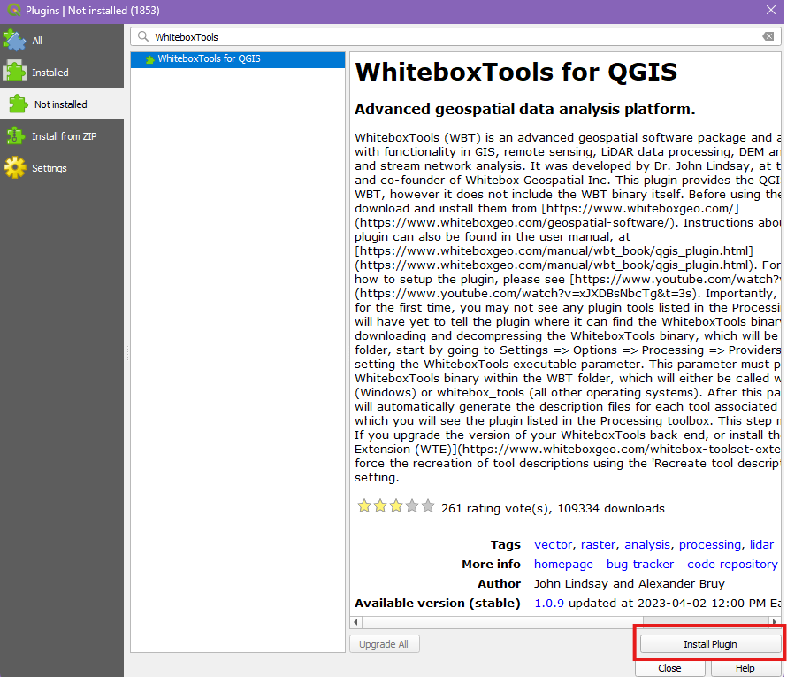
In QGIS, open Plugins → Manage and Install Plugins. In the search bar, type "WhiteboxTools" and the plugin should appear in the list. Select it and click "Install Plugin".

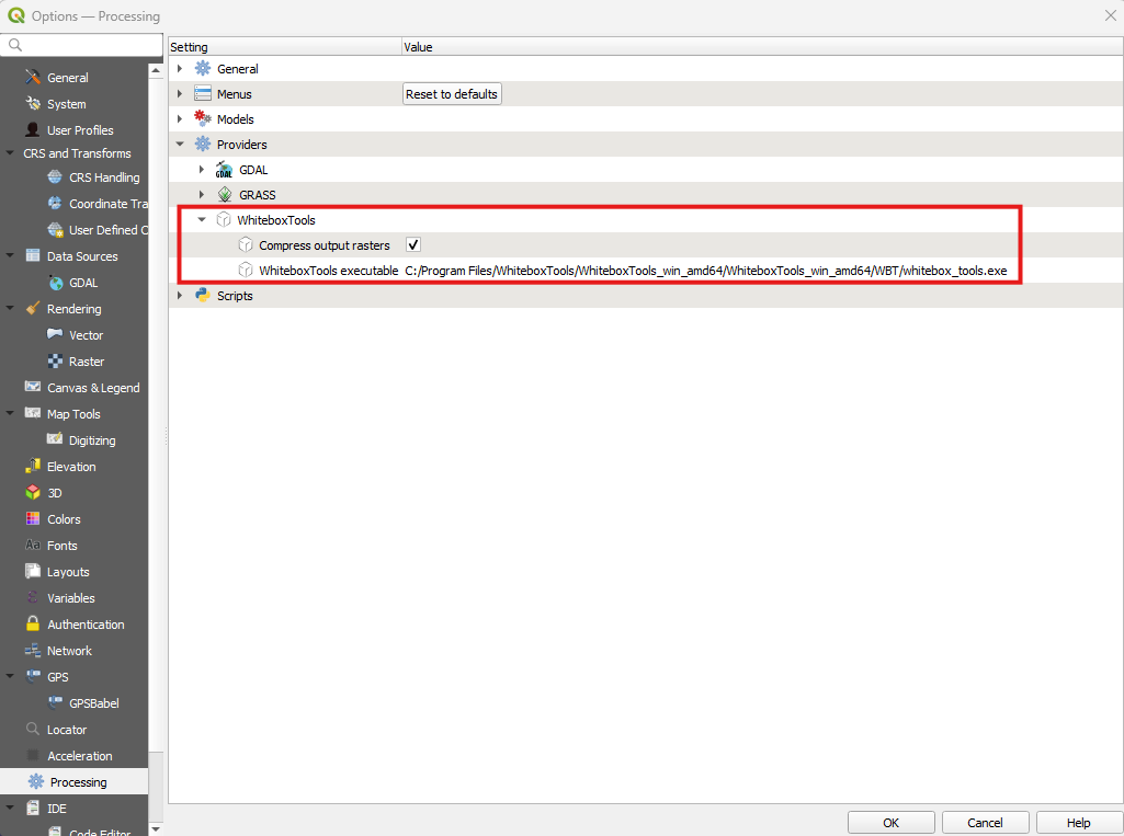
To configure the path to the WhiteboxTools executable, open Settings → Options → Processing. In the dialogue window, open Providers → WhiteboxTools, and under "WhiteboxTools executable", browse to the folder where you extracted the files and select the file named "whitebox_tools" which is found inside the WBT folder.

Once configured, WhiteboxTools tools will appear in the QGIS Processing Toolbox.

Downloading the DEM

The digital elevation model (DEM) used in this tutorial is the Copernicus GLO-30 Digital Elevation Model, downloaded through the OpenTopography portal.

Feel free to use your own DEM, but if you wish to follow the tutorial with the exact dataset shown here, go to the Copernicus GLO-30 Digital Elevation Model.

On the OpenTopography page, scroll down to the "Coordinates" section, check off "Manually enter selection coordinates", and enter the following:

X_min = -115.44776916503906

Y_min = 50.68473994828557

X_max = -115.0165557861328

Y_min = 51.03926216055825

Before submitting the request, ensure the output format is set to "GeoTiff".

Importing the DEM into QGIS & Preparing Your Workspace

Once your DEM has been downloaded, the first step is to load it into QGIS.

You can add the DEM to QGIS by going to Layer → Add Layer → Add Raster Layer. Navigate to your downloaded DEM in the dialogue window and click "Add".

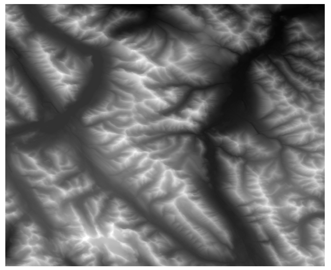
The DEM should now appear as a grayscale raster in the QGIS map window. It should look something like this:

Make sure to rename the DEM layer as well. Meaningful layer names are crucial for an organized workflow, especially in hydrological and/or terrain analysis where many output rasters are generated. Renaming the DEM ensures all subsequent outputs are easy to identify and prevents confusion when selecting inputs for WhiteboxTools tools.

To rename the layer, right click the DEM in the Layers panel and click on "Rename Layer". Choose a meaning full name, such as: "kananaskis_rawDEM".

Before moving on to the next step, ensure you have saved your QGIS project.

Preprocessing

Breaching Depressions

Before running any hydrological tools, the DEM needs to be hydrologically corrected. Raw digital elevation models almost always contain small artificial depressions that happen because of noise, interpolation gaps, or missing elevation values. These depressions trap flow, which prevents tools like D8Pointer and D8FlowAccumulation, both used in subsequent steps, from producing a proper drainage network.

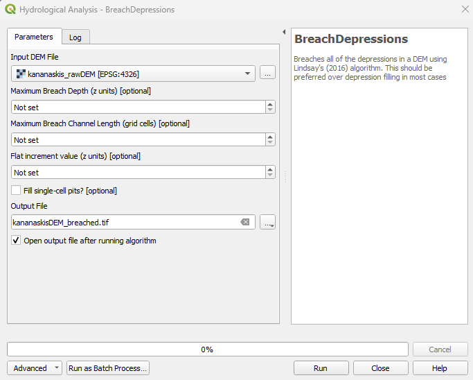
To fix this, we use BreachDepressions in WhiteboxTools, which removes the depressions by cutting narrow channels through them so water can continue flowing downslope.

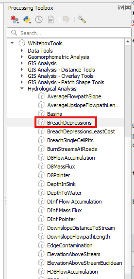
In QGIS, open the Processing Toolbox. At the bottom of the toolbox pane, expand WhiteboxTools → Hydrological Analysis → BreachDepressions.

In the dialogue window, select your DEM as the input. For this tutorial, all parameters are left at their default values. The WhiteboxTools manual explains what each parameter does but it does not require any specific modifications for general preprocessing. Since the goal here is to demonstrate the workflow rather than fine-tuning terrain modifications, the defaults are perfectly fine.

Choose a meaningful output name, such as kananaskisDEM_breached, and remember to add .tif at the end.

A quick note: WhiteboxTools also includes a FillDepressions tool. Both breaching and filling can be used for hydrological correction, but breaching tends to preserve the natural shape of the terrain better, which is helpful for mountain regions like Kananaskis.

Step 3: Hydrological Processing

Flow Direction

Once the DEM is hydrologically corrected, the next step is to calculate flow direction. This tells us the direction water would flow naturally move from every cell in the DEM.

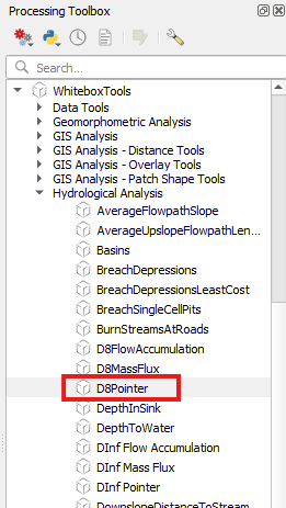
To do this, we will use the D8Pointer tool. The D8 algorithm assigns each cell a direction based on the steepest downhill neighbour. It's simple, efficient, and is the standard method used for most hydrological workflows.

In the QGIS Processing Toolbox, go to: WhiteboxTools → Hydrological Analysis → D8Pointer.

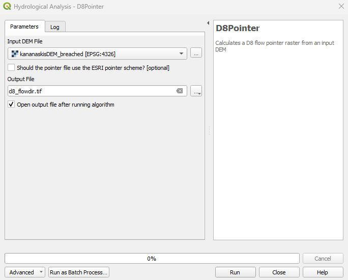
Select your breached DEM as the input and choose a meaningful name for the output file. You may consider d8_flowdir.tif.

Leave the "Should the pointer file use the ESRI pointer scheme?" unchecked. WhiteboxTools uses its own D8 pointer scheme, which is different from the ESRI scheme. Since this tutorial does not require ESRI compatibility, the option is left unchecked. However, if your workflow later requires ESRI compatibility, you may check this option.

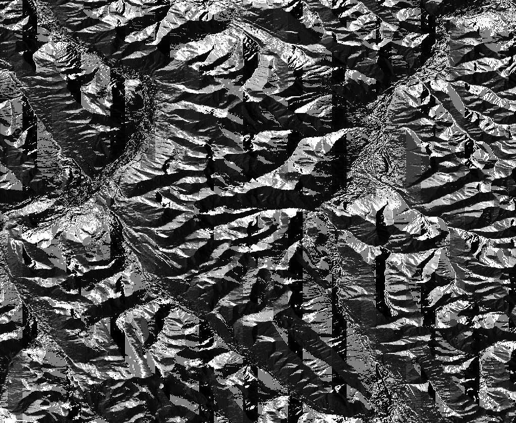
The output should look something like this:

The output may look a bit intense but this is normal. You won't really need to "interpret" it visually, as its main purpose is to feed into the next step.

Flow Accumulation

With flow direction calculated, the next hydrological step is to create a flow accumulation model. Flow accumulation counts how many upstream cells drain into each location, allowing us to visualize drainage density, major channels, and areas prone to runoff.

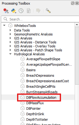
In the QGIS Processing Toolbox, go to: WhiteboxTools → Hydrological Analysis → D8FlowAccumulation.

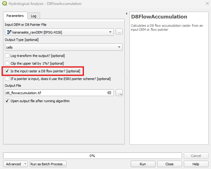
Select your flow direction raster as the input. Make sure "Is the input raster a D8 flow pointer?" is checked, since we are using the pointer output from the previous step, and leave all other parameters at their default values. Give your output a meaningful name, such as, d8_flowaccumulation.tif.

WhiteboxTools offers three output types, but for this tutorial, we will use the default "cells" option, which represents the number of upslope contributing grid cells. All three options are compatible with the Topographic Wetness Index we will do later so there is no need to change it unless the workflow specifically requires a different measure.

The "log-transform output" option was intentionally left unchecked. While WhiteboxTools allows the flow accumulation to be log transformed for visualization purposes, the manual explicilty states that log-transformed accumulation grids should not be used for secondary terrain indices like the Topographic Wetness Index (TWI). Since TWI is part of our workflow, we need the original accumulation values.

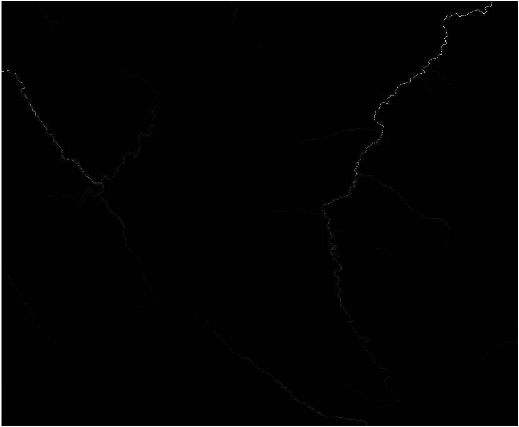
The output will look something like this:

After running the tool, your flow accumulation raster will probably appear almost completely black but this is normal. Flow accumulation usually span a huge range of values (1 to 790430 in this case) and because QGIS applies a simple linear min-max stretch to the raster, the extremely large values dominate the range. When this happens, most cells fall near the darker end of the scale and the drainage network becomes extremely difficult to see until the symbology is adjusted.

Optional: Improving Flow Accumulation Visualization

This step is purely for visualization so feel free to skip it if you wish.

To make the output interpretable:

1. Right click on the flow accumulation layer → Properties → Symbology

2. Change Render type to Singleband pseudocolor.

3. Choose a colour ramp. I chose "Blues."

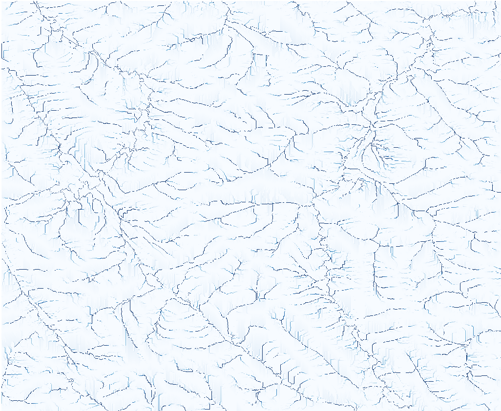
4. Under Min / Max Value Settings, select Cumulative count cut. Selecting this removes extreme outliers from the min/max range. Since flow accumulation contains extremely large values, this option makes the drainage patterns visible by preventing those outliers from influencing the colour stretch.

In addition to these, the brightness, gamma, saturation and contrast can also be adjusted to help with visualization.

After the changes in symbology, the layer should look something like this:

Step 4: Terrain Analysis

Slope

Slope is a basic tool in terrain analysis that describes how steep each cell is. It is required later for the Topographic Wetness Index (TWI), where slope influences how easily water flows downslope. Steeper slopes encourage faster runoff, while gentler slopes promote moisture retention.

WhiteboxTools calculates slope by comparing each cell's elevation to its surrounding neighbours, providing a smooth and realistic steepness estimate across the terrain.

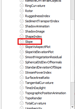
In the QGIS Processing Toolbox, go to: WhiteboxTools → Geomorphometric Tools → Slope.

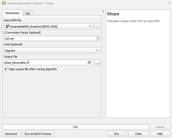
Select your breached DEM as the input and choose a meaningful output name, such as slope_kananaskis.tif.

Leave all parameters at their default values. Since the Copernicus GLO-30 DEM uses metres for both horizontal and vertical units, the "Z Conversion Factor" can be left as "Not set". If you are using a different DEM, make sure the units match, otherwise a Z Conversion Factor will need to be applied.

There is also no need to change the units. WhiteboxTools uses degrees as the default, which is the standard format used across most GIS software. It is also the expected unit for calculating TWI so we don't need to adjust anything, the TWI tool handles any necessary internal conversions automatically.

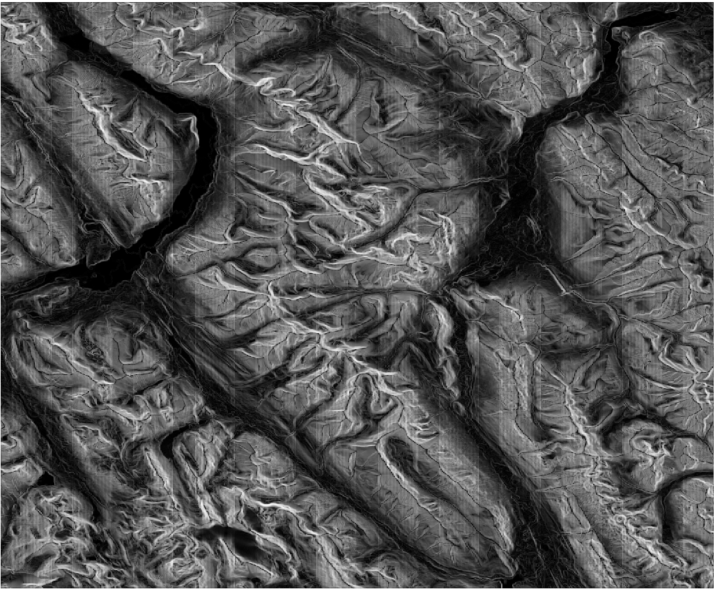
After running the tool, your slope output should look similar to this:

Topographic Wetness Index

The Topographic Wetness Index (TWI) highlights areas where water is more likely to accumulate on the landscape. It combines upslope contributing area with slope to estimate how easily water can pool or saturate a location. Higher TWI values typically indicate wetter, more saturated zones, while lower values identify ridges or well-drained areas.

WhiteboxTools uses two inputs for this step:

• a flow accumulation raster representing the upslope contributing area
• a slope raster measured in degrees

Our workflow already produced both: the D8 flow accumulation (in cells) and the slope raster from the previous step.

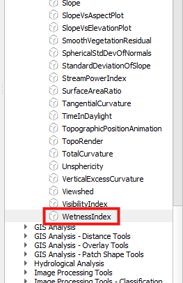
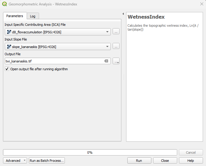
In the QGIS Processing Toolbox, go to: WhiteboxTools → Geomorphometric Tools → WetnessIndex.

Select the following inputs:

• Specific Contributing Area (SCA): your flow accumulation raster
• Slope: your slope raster

Even though the TWI tool refers to "Specific Contributing Area," the default "cells" output from D8FlowAccumulation provides the required upslope area information.

Choose a meaningful output name, such as twi_kananaskis.tif'

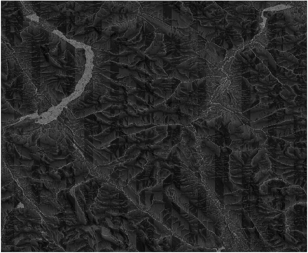
Your output should resemble this:

Visualizing the Topographic Wetness Index (TWI)

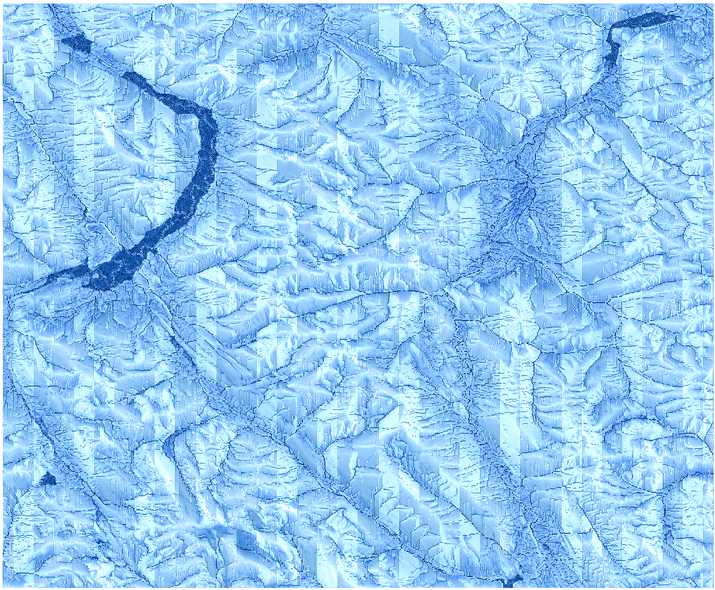
The raw TWI raster will likely appear very dark or low contrast at first. This is normal and expected because the values typically have a narrow range, and without symbology adjustments, the drainage patterns can be difficult to see. Good cartographic practice focuses on communicating spatial patterns clearly so improving the visualization is an essential step in the workflow.

Improving TWI Visualization

To style the TWI output:

1. Right click on the flow accumulation layer → Properties → Symbology

2. Change Render type to Singleband pseudocolor.

3. Choose a colour ramp. I chose "Blues."

4. The brightness, gamma, saturation and contrast can also be adjusted under "Layer Rendering".

The layer with "blues" looked a bit washed so I did make adjustments in the "Layer Rendering." If you wish to follow the exact..., they are as follows:

• Brightness → 0
• Gamma → 0.20
• Contrast → 5
• Saturation → 0

After the changes in symbology, the layer should look something like this:

Optional: Adding Hillshade for Enhanced Terrain Context

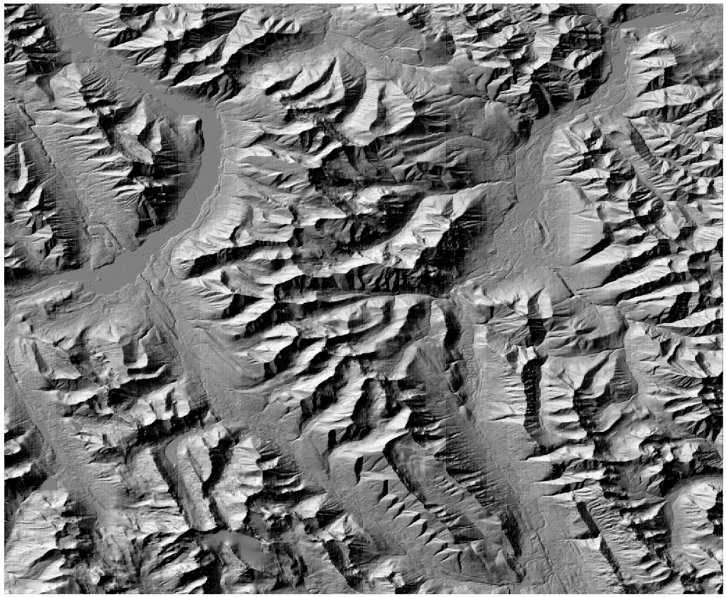
Hillshade is not a requirement in this workflow but placing it beneath the TWI layer with partial transparency can enhance the terrain and make the wetness patterns much easier to see. It also produces a more visually appealing final map.

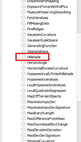
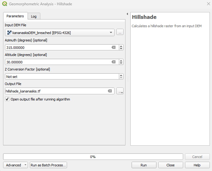
In the QGIS Processing Toolbox, go to: WhiteboxTools → Geomorphometric Tools → Hillshade.

Select your breached DEM as the input and leave all parameters at their default values. Make sure to choose a meaningful output name, such as hillshade_kananaskis.tif.

Your hillshade output should resemble this:

Step 5: Finalizing TWI Visualization

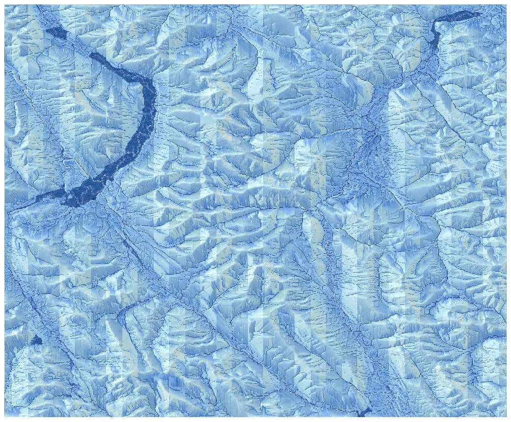
Now that both layers are ready, we can stack them to create the final TWI visualization. Make sure the hillshade is below the TWI layer in the Layers panel.

Right click the TWI layer, open Properties → Transparency and adjust the Global Opacity. Around 80% works well, but you can finetune it depending on your colour ramp and how strong you want the terrain shading to appear.

Lowering the TWI opacity allows the hillshade beneath it to show through just enough to give the map some terrain definition, while still keeping the TWI colours clear and readable.

Your map should now show both the wetness pattern and the underlying landform structure:

Conclusion

At this point, you have taken a raw DEM through every major step of a hydrological and terrain workflow using WhiteboxTools in QGIS. By correcting the terrain, modelling the flow direction and accumulation, deriving slope, and finally calculating and visualizing the Topographic Wetness Index (TWI), you now have a fully processed TWI raster that is ready for mapping or further analysis.

This workflow can be adapted to other regions, resolutions, or hydrological applications and the same tools can be used to dive into more advanced modelling. The hope is that this tutorial not only produced a usable TWI raster but also gave you a clearer understanding of how each WhiteboxTools operation contributes to the final result.

References

• Lindsay, J. B. (n.d.). WhiteboxTools User Manual. Whitebox Geospatial Inc. https://www.whiteboxgeo.com/manual/wbt_book/intro.html
• Whitebox Geospatial Inc. (2025). Whitebox Software. https://www.whiteboxgeo.com/
• QGIS. (2025). QGIS User Guide. QGIS.ORG. https://docs.qgis.org/3.40/en/docs/user_manual/index.html