Cost Path Analysis of Mars using SAGA

Purpose

This tutorial will describe the detailed steps required to perform Cost Path Analysis using SAGA GIS, a free and open source software. It will use SAGA’s Grid tools to perform terrain analysis and basic grid/raster processing using a digital terrain model (DTM) from the surface of Mars, as well as Shape tools for some vector dataset creation. Finally, there will be an introduction to some tools and processes used in more advanced cost-path analysis.

Objective

This tutorial aims to provide step-by-step instructions for completing cost-path analysis within SAGA. The basic analysis will use tools from the following built-in libraries: Grid, Shape and Terrain Analysis. A more advanced analysis will further explore tools within the Grid library. By the end, this tutorial will have shown you how to use SAGA’s built-in tools to perform a cost-path analysis using a Mars DTM and be exposed to more advanced techniques to enhance the basic cost-path analysis.

Introduction

SAGA

SAGA is an open source program for GIS that has a lot of capability in geoscientific analysis and has been designed for effective implementation of spatial algorithms. It features an extensive suite of tools covering raster data (called Grid data within SAGA) and operations, imagery processing, vector processing as well as some ecological and geomorphological simulations, to name a few. More information can be found at their homepage, and the latest version of their software can be downloaded from SourceForce.

Cost-Path Analysis

(insert intro on CPA here, note least cost path we will use)

Background and Data

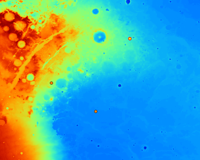
This tutorial will explore Northeast Syrtis, which refers to the northeast segment of Syrtis Planum Major quadrangle, which is a candidate landing spot for the Mars 2020 rover mission. As part of the preparation for the mission, stereo images of the potential landing site were taken by NASA’s Mars Reconnaissance Orbiter. The images were then used to create a digital terrain model (DTM), with the primary objective of being used in the rover mission’s Entry, Descent and Landing (EDL) simulations. The DTM of NE Syrtis (download here) is made available by the USGS Astrogeology Science Center.

For our analysis, we will be using the DTM to determine the path of the rover once it has landed.

Methods

Uploading Data into Saga

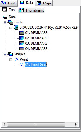
The first step is to upload a DEM into Saga, because this program has very specific file formats that it can handle, a previous tutorial will show how this is done. It can be found within Exploring Hydrological Analyses.

Creating Points

To create points on a layer, go into Geoprocessing>>Shapes>>Points>>Create Point Grid, this will bring up a window.

Save it to where your files are, click okay and a new shape layer will be created within your data window, within that window right click on the "Point Grid" and go into edit and "add shape".

Using the action tool , create points by selecting the location on the map, then right click and click edit selected shape, and apply the changes. To create multiple, right click and add shapes.

Kriging

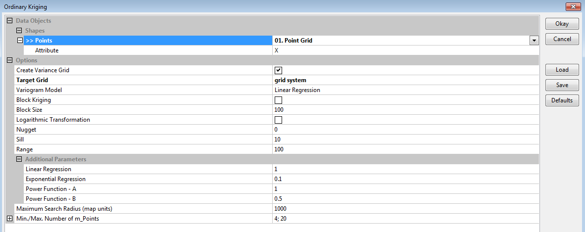
To be able to add the points to a grid layer, Ordinary Kriging will be done. For the uses of different Kriging methods the information can be found at Full Module Index

by going into Geoprocessing>>Spatial and Geostatistics>>Kriging>>Without Variogram Fit>>Ordinary Kriging.

This window should appear; add the point grid created in the "Points" section, also change target grid to "Grid System". Click okay and another window should appear.

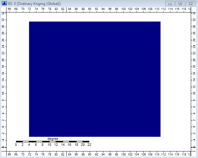
Select the appropriate grid system and select okay and an image should appear.

Terrain Analysis

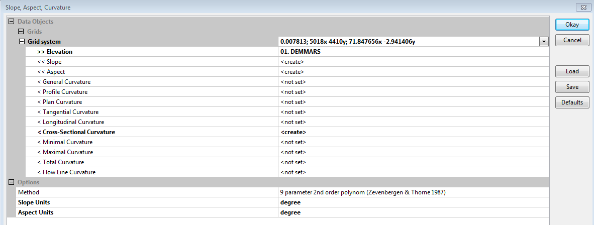
The terrain analysis within Saga has a simple method of selecting any surface that you would like to determine all within one window. By going into Terrain Analysis>>Morhpometry>>Slope, Aspect, Curvature. A window should appear that will give you available options of what processes can be done.

- The Grid layer was selected,

- The DEM elevation was Chosen,

- In the drop down tabs, create was selected beside Slope, Aspect, Cross sectional Curvature

- In methods, a 9 parameter 2nd order polynomial was chosen,

- Slope and Aspect units, where changed to Degrees

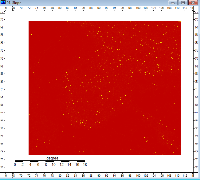
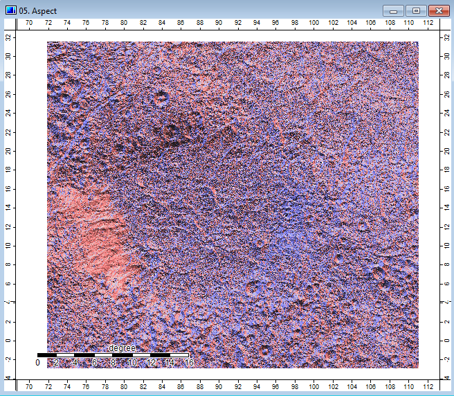
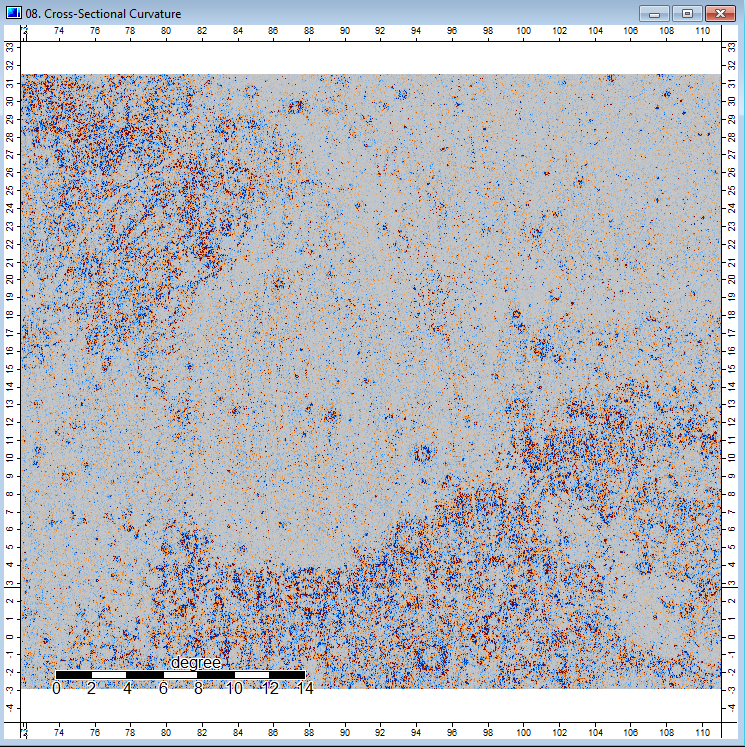
The following three figures were produced by the Terrain Analysis tool.

Figure 1: Slope of Mars Terrain, indicating slope

Figure 2: Aspect of Mars Terrain, showing the location of the aspect

Figure 3: Cross-Sectional Curvature of Mars Terrain

Reclassify

To reclassify the values to set range and remove empty cells, go into Geoprocessing>>Grid>>Values>>Reclassify Grid Values.

- Select the Grid system that needs to be reclassified.

- Select the Grid, the DEM mars is shown, same processes is done with Slope.

- Choose the values that want to be reclassified. In this case 0 to 1.

- No Data value of input can be selected here as well.

Accumulation Cost

An accumulation cost is necessary for Least Cost Path, here the values created above will be used for this step. By going into Geoprocessing>>Grid>>Cost Analysis>>Accumulated Cost(Isotropic) within this window:

- Set the Grid system

- The Cost Grid, in this case the reclassified slope layer

- Set the destination points, the Kriging of the points

- The threshold for destination route, 0 was selected

- Ensure that you create an accumulation cost and Closest point

Least Cost Path

Finally, finish the least cost path, by going into Geoprocessing>>Analysis>>Cost Analysis>> Least Cost Paths;

- Select the grid system

- Within Accumulation Cost use the Accumulation Cost layer created above,

- Within Values select the nessecary values, in this case Slope was chosen.

- The source points are the original point layer created at the begining of this tutorial

More in depth research required

To fully understand what is happening and what selected process would work best for your DEM, readings should be done to see what each tool is and how to work on your selected file Full Module Index, as well as aids from other tutorials preforming a different method of cost path.

Conclusion

This tutorial showed the basic steps that are needed to perform a cost path analysis. However, due to issues with the coordinate systems within SAGA, where planetary bodies such as Mars have yet to be given a Projected Coordinate system, these cost path analysis could not be completed. This does leave room for more updates to be installed and possibly an update package that can include more processes for other worlds, such as change coordinate systems, measure distances with existing Coordinate systems. Other than that, this program offered simple and effective method of terrain analysis, and Kriging Points to a surface.

References

Sohail Dham and Colin Doucette. Exploring Hydrological Analyses, http://gracilis.carleton.ca/CUOSGwiki/index.php/Exploring_Hydrological_Analyses_using_SAGA_GIS/

Saga Library website, http://www.saga-gis.org/saga_module_doc/2.1.3/a2z.html

Saga Cost Path, http://sourceforge.net/projects/saga-gis/files/SAGA%20-%20Documentation/Tutorials/Least_Cost_Path_Analysis_Tutorial/

Kim Cimmery(2013),Tutorial: Using SAGA for Least Cost Path Analysis,http://download2.polytechnic.edu.na/pub4/sourceforge/s/sa/saga-gis/SAGA%20-%20Documentation/Tutorials/Least_Cost_Path_Analysis_Tutorial/LCPAtutorial.pdf