Georeferencing Raster Imagery in SAGA GIS

Introduction

Georeferencing

Raster data produced by scanning aerial photographs, toposheets, or print maps normally do not contain any spatial reference information. Other times, the image does not properly align with other data, and requires transformation in order to be used in conjunction with existing data. Georeferencing rasters is a means of accomplishing both courses of action, and is a common and important task in the field of geospatial analysis (especially when working with historical imagery or maps). ESRI defines Georeferencing as:

Aligning geographic data to a known coordinate system so it can be viewed, queried, and analyzed with other geographic data. Georeferencing may involve shifting, rotating, scaling, skewing, and in some cases warping, rubber sheeting, or orthorectifying the data. citation

This tutorial contains an introduction to the process of georeferencing imagery in the SAGA GIS software, as well as information on the fundamentals of the georeferencing process.

SAGA GIS

Figure 1: SAGA GIS Logo

For the following tutorial, System for Automated Geoscientific Analyses, or SAGA GIS software will be used. SAGA GIS is a free, open-source geographic information system program, originally developed by a small team of researchers from the Department of Physical Geography in the University of Gottingen, Germany.When the SAGA GIS team began development in 2001, the purpose of the software was aligned with the needs of the development team, such as the analysis of raster imagery, with a focus on digital elevation models (DEM). SAGA has also been designed for an easy and effective implementation of spatial algorithms. Over the years, however, the software has broadened in scope, as it has seen many feature contributions from its world-wide user community. Interestingly, the users have freedom of improving the program, modifying it and releasing the improvements to the public. This resulted in a comprehensive, growing set of geo-scientific methods combined an easily approachable user interface with many visualization options. The software is available for Windows, Linux, and FreeBSD operating systems. (http://www.saga-gis.org/en/index.html)

Features

• Object oriented system design (C++)
• Modular structure allows framework independent function development
• SAGA API with immense support for geodata handling
• GUI for intuitive data management, analysis and visualization
• Runs on Linux as well as on Windows operating systems
• Portable software running without installation even from memory sticks (MSW)
• Free and Open Source Software (FOSS)
• Scripting via command line, Python, Java, R
• Far more than 450 freely available functions for geodata analysis
• Georeferencing and cartographic projections
• Grid interpolation of scattered point data, triangulation, IDW, splines, ...
• Vector tools: clipping, buffer zones, raster to vector conversion, ...
• Image analysis: filters, supervised classification, PCA, FFT, OBIA, ...
• Geostatistics: GWR, variograms, ordinary & universal Kriging, ...
• Terrain analysis: morphometry, hydrology, illumination, classification, ...
• and many more ...

Installation Instructions

The latest version of SAGA GIS can be downloaded on the SAGA GIS Sourceforge page. At the time of writing, the latest version of SAGA GIS is 6.4.0. Documentation for the SAGA GIS tool library can be found in the SAGA-GIS Tool Library Documentation

Data Acquisition

For the following tutorials, you will need to acquire imagery from two sources: Satelite imagery from Google Earth, and a PDF toposheet or scanned print map.

Google Earth

For this tutorial, we will be using imagery from google earth. to obtain this imagery, perform the following steps.

1. ensure that you have downloaded and installed Google Earth on your computer
2. Open Google Earth, and zoom to the area of interest of your choice. for this tutorial, we used the area around the Smithsonian Museum of Natural History in Washington, DC, USA, but any location will suffice.
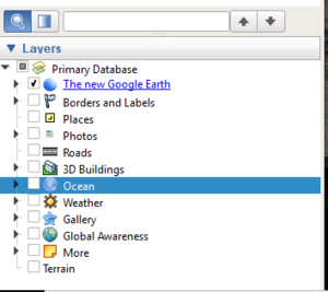
3. In the Layers menu in the bottom left corner of your screen, uncheck all layers. Google earth renders terrain in 3d, and the perspective this creates can distort your exported imagery (See Figure 2).
   
   
   

   Figure 2: Layers Menu of Google Earth
   
   
   
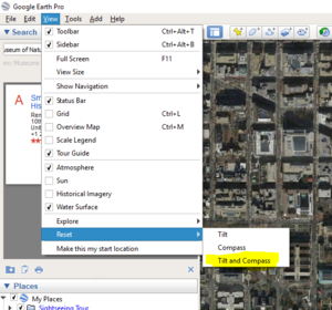
4. Ensure that your imagery is north-facing and vertically-angled by selecting View -> Reset -> Tilt and Compass in the menu bar at the top of the screen (See Figure 3)
   
   
   

   Figure 3: Resetting the Angle and Rotation of Google Earth
   
   
   
5. Under Tools -> Options, ensure that under Show Lat/Long, Universal Transverse Mercator is selected.
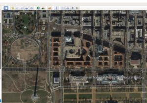
6. Using the Add Placemark tool (See Figure 4), add four or more placemarks to your screen. make note of their coordinates and label them numerically. change their icon to one that is more precise, location-wise.
   
   
   

   Figure 4: Adding Placemarks in Google Earth
   
   
   
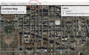
7. Save your image by selecting File -> Save -> Save Image in the menu bar at the top of the screen. then, press the Save Image Button (See Figure 5).
   
   
   

   Figure 5: Saving Your Image
   
   
   

Print Map

For this tutorial, we will be using a scan of a historical watershed boundary map of Alberta, made available through the Open Government License. the following pre-tutorial steps must be performed:

1. Download the file from the following link. you can use any other PDF or raster map as long as it contains some sort of absolute location information.
2. If necessary, convert the pdf to a raster TIF file. many free websites exist to perform this conversion, such as PDFaid.com. Ensure that the conversion is performed at a high enough DPI that all text is legible. for this tutorial, we chose 150 DPI.
3. Save the converted file in a working directory of your choice.

Tutorial

Georeferencing a Historical Map

In the following tutorial, the process of georeferencing a historical map in SAGA GIS will be explained. To begin, we will import the image into SAGA GIS.

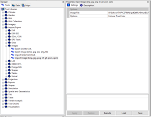
1. In the Tools tab, select Import/Export -> Images -> Import Image
2. In the Image File field, select the historical map you downloaded earlier
3. In the Options field. select Enforce True Colour
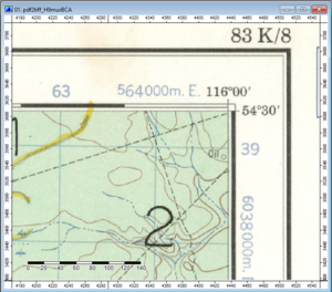
4. Double click your imported file in the Data Tab in order to view the file.
   
   
   

   Figure 6: Importing Imagery into SAGA GIS
   
   
   

Creating Ground Control Points

In order to georeference an image, we use Ground Control Points (GCPs). these are points that establish a relationship between the pixel coordinate system of the raster to a coordinate system of the earth. GCPs are typically placed at sharp features such as intersections or easily visible landmarks, but for this map, we will use sections of the map graticule with known coordinates.

1. To start creating the GCPs, we will run the Create Reference Points module. in the Tools tab, select Projection -> Georeferencing -> Create Reference Points [Interactive]'.
2. Click the Okay button in the pop-up menu. this module creates a shapefile with two attribute fields, used to store the latitude and longitude of a point.
3. Zoom to an area of the imported file with known coordinates, such as the intersection of two known graticules (See figure 7).
   
   
   

   Figure 7: Initial GCP Location
   
   
   
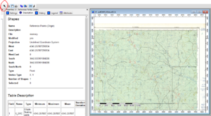
4. Select the Action button (See figure 8), and click the location of your first GCP. in the pop-up window, enter the x and y (on earth) coordinates of that point.
   
   
   

   Figure 8: Action Button
   
   
   
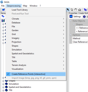
5. Repeat this process at least four more times, each with a different point. Once you have completed this, end the module by selecting Geoprocessing -> Create Reference Points [Interactive] in the menu bar at the top of the screen (See figure 9).
   
   
   

   Figure 9: Ending a Module
   
   
   

Defining Projection

We must now add projection information to the image. According to our map, the projection used is NAD 1927 UTM.

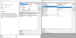
1. Open the Set Coordinate Reference System module. in the Tools tab, select Projection -> Proj.4 -> Set Coordinate Reference System. Select the User Defined field, and in the popup menu, change the Projection Type field to Universal Transverse Mercator (UTM). in the Predefined Datum Field, select North_American_Datum_1927. In the popup menu, press Okay. (See Figure 10
   
   
   

   Figure 10: Setting a Coordinate System
   
   
   
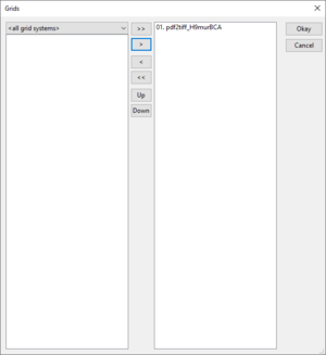
2. In the module menu, under the Data Objects section, select the Grids Field. A popup menu will open up. Select your image file and click the > button to transfer it to the right side of the popup menu. Click Okay to finish. (see Figure 11)
   
   
   

   Figure 11: Selecting a grid in the Data Objects Menu
   
   
   

Georeferencing the Grid

We now possess all the necessary components to Georeference the map.

1. Open the Rectify Grid module. in the Tools tab, select Projection -> Georeferencing -> Rectify Grid.
2. In the Reference Points (origin) Field, select your generated GCP shapefile. in the Grid System Field, select the grid system of your imported map. In the Grid field, select your imported image (make sure it is the one that you defined a projection for). In the Method field, select Automatic (these choices will be explained in the following tutorial). in the Resampling field, select Nearest Neighbour.
3. A popup menu will open up. set the Cell Size field to 1 (or whatever resolution you desire).
4. In the popup menu, press Okay
5. To save your georeferenced image, in the Data tab, right click the image and press Save As.

Congratulations, you have just georeferenced a map in SAGA GIS!

Georeferencing Google Earth Imagery

The process for georeferencing google earth imagery is very similar to georeferencing a historical map or topo sheet. The main differences are as follows:

1. Instead of using graticles for the GCP locations, use the points you created in google earth when collecting the image
2. Google earth uses the WGS84 Datum and the Equidistant Cylindrical (Plate Caree) Projection. Make sure to use these when defining a projection.
3. Google Earth imagery is NOT orthorectified. If you have any points of known location you can use as GCPs, you may want to, as well as a comparison with LANDSAT imagery if possible.

Transformations and Interpolation

Transformations

Because images obtained from aerial photography may be distorted, often it is necessary to apply a Transformation during the georeferencing process. Different transformations are available at the following transformations are available in SAGA GIS

Triangulation

There is no documentation as to which transformation this represents located anywhere online or otherwise

Spline

Spline transformations are optimized for local accuracy at the expense of global accuracy. In a spline transformation, source and target control points are mapped to each other exactly, while pixels that are further away have greater chance of inaccuracy.

This transformation, known as a "rubber sheet" transformation, is of greatest use when the exact location of certain points is of high importance.

Spline transformations require a minimum of 10 GCPs, and adding more points increases the accuracy of a spline transformation

Affine

Affine is a linear transformation that can scale, translate, rotate, and skew an image. An affine transformation generally maintains straight lines, with squares and rectangles becoming parallelograms.

An affine transformation requires at least 3 GCPs, with each additional GCP introducing additional error. However, inaccurate positioning of GCPs has a greater impact on inaccuracy than additional GCPs, therefore more than 3 GCPs should be used.

First Order Polynomial

This option represents similarity transformations, which are similar to affine transformations in that they are linear, 1st order transformations. however, unlike affine translations, similarity transformations are unable to either independently scale the axis or apply any skew. This is useful for the digitization of "as built" schematics.

A similarity transformation requires 2 GCPs. Additional GCPs will produce RMS error

Second Order Polynomial

Second order polynomial transformations, or quadratic transformations, begin to introduce curvature into the shape of the transformed image. citation a 2nd order polynomial transformation applies a simple global curvature to the raster. Citation

A second order polynomial requires 6 GCPs

Third Order Polynomial

Third order polynomial transformations, or cubic transformations, introduce more complex curvature into the shape of a transformed rasterm citation.

A third-order polynomial transformation requires 10 GCPs.

Polynomial, Order

This setting allows you to input a custom order for your polynomial transformation, increasing the complexity of the curve produced

Resampling

When a geometric transformation is applied to a raster, the cells of the input and output rasters rarely line up. To assign values to each output cell, an interpolative algorithm is applied to the input raster, which then assigns values to the initially-empty cells of the output raster. There are 4 methods of interpolation available for resampling in SAGA GIS.

Nearest Neighbour

Nearest Neighbour assigns to the cell of the output raster the closest cell on the input raster to the corresponding output raster cell.

Values in the input raster directly correspond to values in the output raster. there are no changes made to any input raster values.

This method is suitable for nominal and ordinal data, as if the input raster is entirely integer, so too will the output raster. As such, catergories and classes are maintained

Bilinear Interpolation

Bilinear interpolation assigns to the output raster the average of the 4 nearest cells on the input raster to the corresponding output raster call. the average value is weighted to account for distance, with closer cells having relatively more influence than more distant cells.

Bilinear interpolation is valuable for continuous data as it produces a much smoother surface than Nearest Neighbour or Bicubic Spline interpolation.

Bicubic Spline Interpolation

Bicubic Spline interpolation, also known as cubic convolution, assigns to the output raster the distance-weighted average of the nearest 16 cells of the input raster to the corresponding output raster cell.

As more cells are included in the weighted average, the results are sharper and therefore more suited to satelite and aerial photography.

For the same reasons as Bilinear Interpolation, Bicubic Spline interpolation should not be used for categorical data.

citation.

B-Spline Interpolation

B-spline interpolation makes use of a sequence of increasingly fine-scale bicubic functions to approximate the function of a single B-spline function. This functions similarly to B-spline interpolation, but is more computationally efficient. citation