R Studio's Spatial Capabilities

Purpose

This tutorial prominently centers on the abilities of R Studio; an open source software program utilizing the programming language 'R' which is often used for data analysis, statistics and the graphing of very large data sets. Users may want to view spatial output of their data and R has a package (sp) that allows for the manipulation of spatial data. If users are not familiar with the package, then they may want to import the data to more visual software such as QGIS. QGIS uses the scripting language Python. In order for R and QGIS to communicate the scripting language must be translated.

This tutorial shows how one could manually translate Python to R language - this required knowledge of how both programs operate, and how to use spatial packages in R Studio.

Introduction

How to use R Studio:

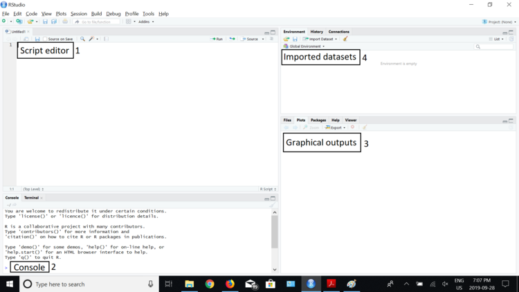
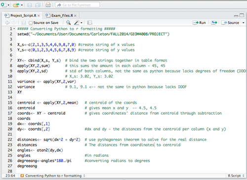
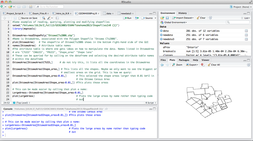
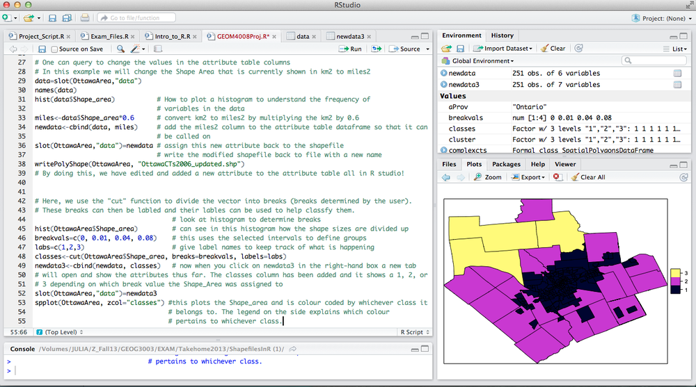
Figure 1: The top left-hand box (1) is the script editor. This is where one inputs all their commands; how to manipulate the data, perform analysis, and create graphical outputs. The bottom left-hand box (2) is the console. This is where commands can be written, but these will not be saved if the GUI (Graphical User Interface) closes, and results are shown. When one runs a command in R Studio, the command along with its output is shown in this section, unless it is a plot. The bottom right-hand box (3) is where graphical outputs are shown, and where help files, packages and data files can be found. The top right-hand box (4) shows datasets that have been imported and keeps track of data and values that have been assigned in your R scripts. One can click on the datasets to view them in a table format in another window.

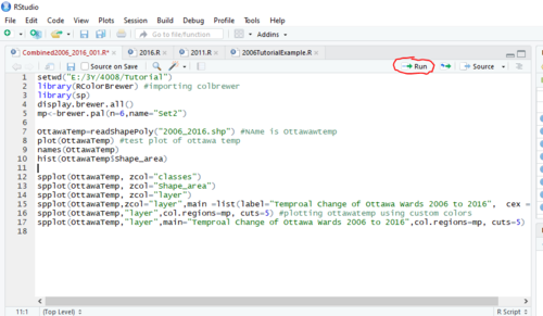
In the command console one can simply type the command and press 'Enter' and the command will go through right away. In the script editor one can type their command or as many as they wish, and then run it by selecting the line(s) they wish to run and clicking 'Run' - a button located in the upper right-hand corner of the script editor (As can be shown below in Figure 2.)

Figure 2

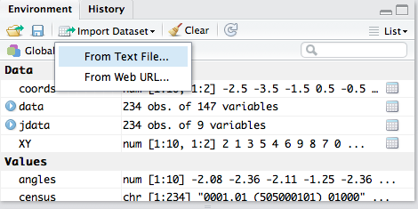
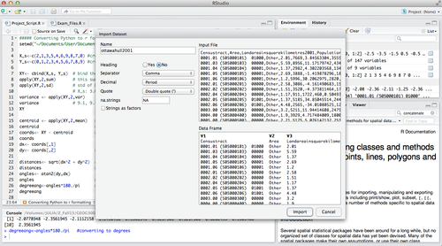
Often one has large datasets that they wish to analyze. The datasets can be imported via text and .csv files, either by selecting "Import Dataset" on the R Studio GUI or by entering a command line such as: insertnamefordata <- read.csv("/User/Documents/YOURDATA.csv"). Entry by command line requires one to know the exact path to the dataset.

Figure 3

Figure 4

As shown in Figure 4, one can decide what to name the dataset there importing and how to arrange it in the most suitable way. Generally one renames their data, adds headers, separates by comma, and leaves the rest as default.

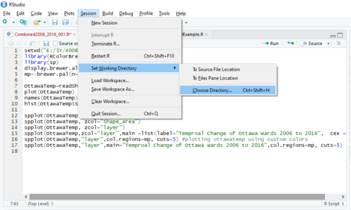
One should also set a 'working directory'; this is a folder where all data can be located and where the '.R' file will be saved. This can be done by clicking 'Session' in the top tool bar of the R Studio GUI, selecting 'Set Working Directory' and then 'Choose Working Directory' and navigating to the correct folder, as shown in Figure 5.

Figure 5

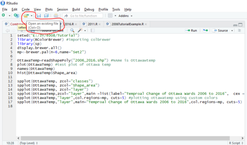
For data analysis, one can import a script that someone has already created, or import one that they were previously working on. This is done in the top left-hand corner with the open folder icon(See Figure 6). Then one can rename the data according to how they imported their own. One would then have to go through the pre-made script and insert the proper name for the data accordingly. Another method is to write the script yourself depending on how much you know about the language and want to customize the process for a specific purpose.

Figure 6

Methods

A Comparison

Commands in Python

Command in R Studio in order to achieve the same result

A useful resource for translating between languages is this website: http://mathesaurus.sourceforge.net/r-numpy.html

Spatial R Packages

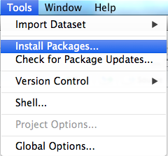
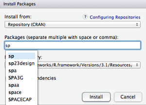
Packages can be installed through the GUI.

Then in the script editor one must type "library(InsertPackageName)" in order to call on the package.

R has packages maptools and sp that allow for manipulation of shapefiles. These packages allow shapefiles (lines, points, polygons and grids) to be read into R and displayed visually in the bottom right-hand corner of the GUI under "plots". The data used for this tutorial is Ottawa Census Data from 2006 that can be found on Carleton's Library website Ottawa Gatineau Census Data.

The following tutorial of Maptools has been modified from Murray Richardson's code and explanation on how to use the tool for spatial manipulation, from his GEOG 3003 course.

Results

A Comparison

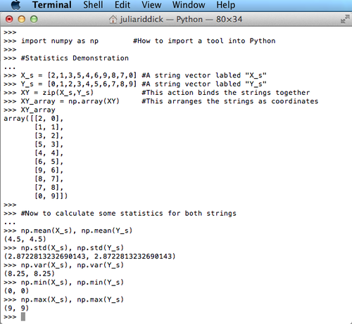
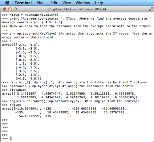
Exact translation between the two languages is almost possible. The biggest issue found is that R did not arrange the XY points as coordinates like they were meant to be. However the results calculated were the same in the end despite R being unable to pair them. When the standard deviation and variance were calculated for the X and Y columns the values were different because in Python there is 1 degree of freedom accounted for. There must be a function in R that allows one to designate the desired degrees of freedom, so finding a solution should not be too difficult.

Spatial R Packages

This tutorial showed a sample of how one can manipulate shapefiles in R without having to export to another software to see the visual representation. The main commands to remember are to concatenate the newly developed or adjusted data to the original shapefile so that it can be re-written Example: classes<-cut(OttawaArea$Shape_area, breaks=breakvals, labels=labs) <-- This is the new data slot(OttawaArea,"data")=newdata3 <-- This adds the new data into the main dataframe writePolyShape(OttawaArea, "OttawaCTs2006_updated.shp") <-- This command re-writes the shapefile to include the latest updates

Another key feature in R Studio is that In the bottom right-hand quadrant where the plots are shown, one can export the images as a .JPEG or .PDF. This is very useful for reports.

References

Acknowledgements

Dan Patterson served as main script editor for anything Python-related Murray Richardson's script with MapTools was from the GEOG 3003 course. This script was instrumental in creating the tutorial.

References

Harris, R. (2011). Statistics for Geography and Environmental Science: An Introduction to R. Http://www.social-statistics.org

Ottawa Gatineau Census Data.

Translating R and Python