Difference between revisions of "Flood Risk Assessment in QGIS"
(→Result) |
(→Data: Added a phrase to prevent reader from immediately going to Open Data Canada and trying to figure out how to download without realizing there are instructions provided further below.) |
||
| (64 intermediate revisions by 2 users not shown) | |||
| Line 1: | Line 1: | ||
==Introduction== |
==Introduction== |
||
Flood assessment is one of many |
Flood assessment is one of many practical applications of GIS. This analysis will focus on the city of Peterborough, a small city northeast of Toronto. The analysis is particularly relevant due to past flooding events in the Peterborough area. By a completing flood risk assessments, the city can identify at-risk infrastructure and populations, as well as develop stronger preparedness measures for future flooding events. |
||
The purpose of this tutorial is to provide users with an introduction/guidance in completing a flood risk assessment, as well as an introductory glance into QGIS. |
|||
The purpose of this tutorial is to provide users with guidance in completing a flood risk assessment, as well as an introductory glance into QGIS. |
|||
==Software Requirements== |
==Software Requirements== |
||
In order to begin this tutorial, |
In order to begin this tutorial, you will need to download the QGIS software package from the following link (https://www.qgis.org/en/site/ ). This tutorial was created using QGIS version 3.8.1. The latest version of QGIS is freely available for Windows, MacOS X, Linux and Android. |
||
All steps of the tutorial will be completed using this free and open source software, and will not rely on the use of any other programs. |
All steps of the tutorial will be completed using this free and open source software, and will not rely on the use of any other programs. |
||
==Data== |
==Data== |
||
The primary source of data used for this analysis will be the High Resolution Digital Elevation Model (HRDEM) - CanElevation Series, produced by Natural Resources Canada for the city of Peterborough. The dataset is hosted on the Open Data Canada website here: (https://open.canada.ca/data/en/dataset/957782bf-847c-4644-a757-e383c0057995); specific download instructions are provided in the next section, below, but first we'll review different forms of elevation data models. |
|||
The primary source of data used for this tutorial can be found in the next section ('''Downloads''') and includes LiDAR data (.tif) for the Ottawa-Gatineau Region in 2014. For the purposes of this analysis, four adjacent elevation tiles will be downloaded, creating a 2x2 grid of raster layers that can be imported directly into QGIS. |
|||
Additional data that will be used includes city of Ottawa 1:25,000 Scale Topographic map, which will consist solely of vector data, downloaded as .shp files. In addition to the major waterways, roads and building data, this dataset also provides contours, airports, railroads, etc.; but for the purpose of this tutorial, please use ‘Major_Water.shp’; ‘Roads.shp’; and ‘Buildings.shp’. |
|||
There are two main types of elevation datasets provided as part of the High Resolution Digital Elevation Model (HRDEM). Both datasets have been derived from airborne LIDAR data. |
|||
*''See next section for instructions on how to download the files''. |
|||
The two datasets are in the form of a Digital Surface Model (DSM) and a Digital Terrain Model (DTM). It is important to know the difference between these two elevation datasets and how this can affect your analysis of flooded areas. |
|||
A Digital Surface Model or DSM is very similar to that of a Digital Elevation Model (DEM) or Digital Terrain Model (DTM). All three show elevation data of the earth’s surface relative to sea level. One major distinction between a DSM and a DTM is the presence of man-made and natural features. The DSM shows the tops of buildings, houses, highways, tree canopies, vegetated surfaces and all manor of other solid features above the surface of the ground. They are traditionally in the form of a raster image. DSM’s are generally used for purposes where it is necessary to see objects protruding from the surface of the earth. This includes tasks such as assessing the encroachment of vegetation or viewshed analysis for a new High-rise <ref>''[https://gisgeography.com/dem-dsm-dtm-differences/ GISGeography]'',Retrieved: 2019-09-21 </ref> |
|||
. They are not used for hydrologic modelling such as a flood analysis. |
|||
A Digital Elevation Model or DEM does not include features that protrude from the ground. A DEM represents the ground elevation from sea level. Therefore, the tops of trees, buildings and other features have been removed to reveal the ground underneath. This is very useful for the purpose of hydrologic mapping, such as flood analysis. DEM’s are generally in the form of a raster image <ref>''[https://gisgeography.com/dem-dsm-dtm-differences/ GISGeography]'',Retrieved: 2019-09-21 </ref>. |
|||
A Digital Terrain Model or DTM can have varying definitions. In some cases, Digital Terrain Model and Digital Elevation Model are used interchangeably. This means that the DTM dataset would be a raster image of the Earth’s surface excluding buildings and vegetation. In other cases, a Digital Terrain Model can be essentially a DEM represented through point data. The dataset shows the elevation of the earth’s surface through a series of equally spaced points (although, in older datasets these points can be unevenly spaced). These points have an associated x and y value along with a third value for elevation. In this case the DTM would be in the form of a vector dataset, such as a shapefile <ref>''[https://gisgeography.com/dem-dsm-dtm-differences/ GISGeography]'',Retrieved: 2019-09-21 </ref>. |
|||
The DTM dataset available through the High Resolution Digital Elevation Model link is in the form of a geotiff (.tif). This means it is essentially the same as a DEM and can be used for our flood mapping analysis. The DTM data that we will be using in this analysis will be at a resolution of 1m and will be projected in the UTM NAD83 (CSRS) coordinate system. |
|||
Additional vector data will also be used in this analysis from the Peterborough Open Data Hub. This includes building footprints, roads, pedestrian footpaths and hydrography polygons. |
|||
*''See next section for instructions on how to download the files''. |
|||
==Downloads== |
==Downloads== |
||
;''' |
;'''Peterborough Digital Terrain Model Data''' |
||
: '''High Resolution Digital Elevation Model (HRDEM) - CanElevation Series''' |
|||
: https://library.carleton.ca/find/gis/geospatial-data/ottawa-lidar |
|||
: ''The High Resolution Digital Elevation Model (HRDEM) - CanElevation Series dataset hosted on the Open Canada Data web portal, where you can download different sets of DTM and DSM data across Canada'' |
|||
: 1. Click on the following [http://ftp.maps.canada.ca/pub/elevation/dem_mne/highresolution_hauteresolution/dsm_mns/1m/ON/2016-17-Peterborough/utm17/ link]. This will take you to the directory where all of the DTM data is stored for the UTM 17 Zone. |
|||
: 1. Click on the link |
|||
: 2. Navigate to '''Layers''' -> Select '''2014 Ottawa LiDAR Index''' -> Zoom in to the downtown core (as seen in the image below). |
|||
: 3. Download the four tiles centered in the screenshot ''(Tiles numbered: '''365_5031''', '''366_5031''', '''365_5030''', and '''366_5030''')''. The numbers can be seen when the tiles have been selected. |
|||
: 4. Click '''Direct Download TIF file''' -> login to your Carleton account -> Extract the files into a single file, where all other files will be stored for the tutorial. |
|||
: 2. Use the find function (Ctrl + F) to find each of the three images listed below in the file directory. |
|||
::1m_utm17_e_20_90 |
|||
::1m_utm17_e_21_90 |
|||
::1m_utm17_e_21_91 |
|||
: 3. Download each file into a folder on your computer. This will be a working folder for all of your flood analysis data. |
|||
[[File:LiDAR.JPG|700px]] |
|||
;'''Peterborough Vector Data ''' |
|||
;'''Ottawa 1:25,000 Scale Topographic Map''' |
|||
: ''This data is hosted by Peterborough's GIS Open Data initiative on their Open Data web portal.'' |
|||
: https://library.carleton.ca/find/gis/geospatial-data/ottawa-125000-scale-topographic-maps/ |
|||
: 1. Click on the following links and download the data as .shp files (a .zip file will be downloaded) |
|||
: 1. Click on the link |
|||
: 2. Select '''Direct Download'''. |
|||
::[http://data-ptbo.opendata.arcgis.com/datasets/hydrography-polygon?geometry=-78.665%2C44.246%2C-78.012%2C44.332 '''Hydrography Polygons:'''] ''This is a polygon of all the waterways in Peterborough. '' |
|||
: 3. Extract the folder ''Map25000' into the same folder as the previous step (keep it in a subfolder) |
|||
::[http://data-ptbo.opendata.arcgis.com/datasets/building '''Buildings:'''] ''This is a polygon layer of all the building footprints in Peterborough.'' |
|||
::[http://data-ptbo.opendata.arcgis.com/datasets/roads '''Roads:''' ] ''This is a line layer of all the road networks in Peterborough.'' |
|||
::[http://data-ptbo.opendata.arcgis.com/datasets/pedestrian-network-polygon '''Pedestrian Network Polygon:''' ] ''This is a polygon layer of all the pedestrian footpaths and bike trails in Peterborough. '' |
|||
: 2. Go to the .zip files you previously downloaded and extract them to the same folder as you Peterborough DTM data. |
|||
==QGIS Methods and Instructions== |
==QGIS Methods and Instructions== |
||
| Line 44: | Line 68: | ||
===Importing and Merging=== |
===Importing and Merging=== |
||
'''Step 1.''' |
'''Step 1.''' |
||
*Open Qgis. |
|||
*Upload the .tif files into QGIS by navigating through the '''Browser''' window. |
|||
*Upload the .tif DTM images in QGIS by clicking on the '''Data Source Manager '''button [[File:Datasource_Manager_Button.png|32px]]. The Data Source Manager window will then appear. |
|||
*Select the folder where your files are saved, (can be added to favourites by right clicking the folder) and drag in all four .tif files to the main window. |
|||
*Select the folder where your files are saved, (this folder can be added to your favourites by right clicking the folder and adding it to your favourites) drag in all four .tif files to the main window (ignore the .tif.ovr files and only use the .tif files). Alternatively, you can double click each file separately to add them to the project one by one. |
|||
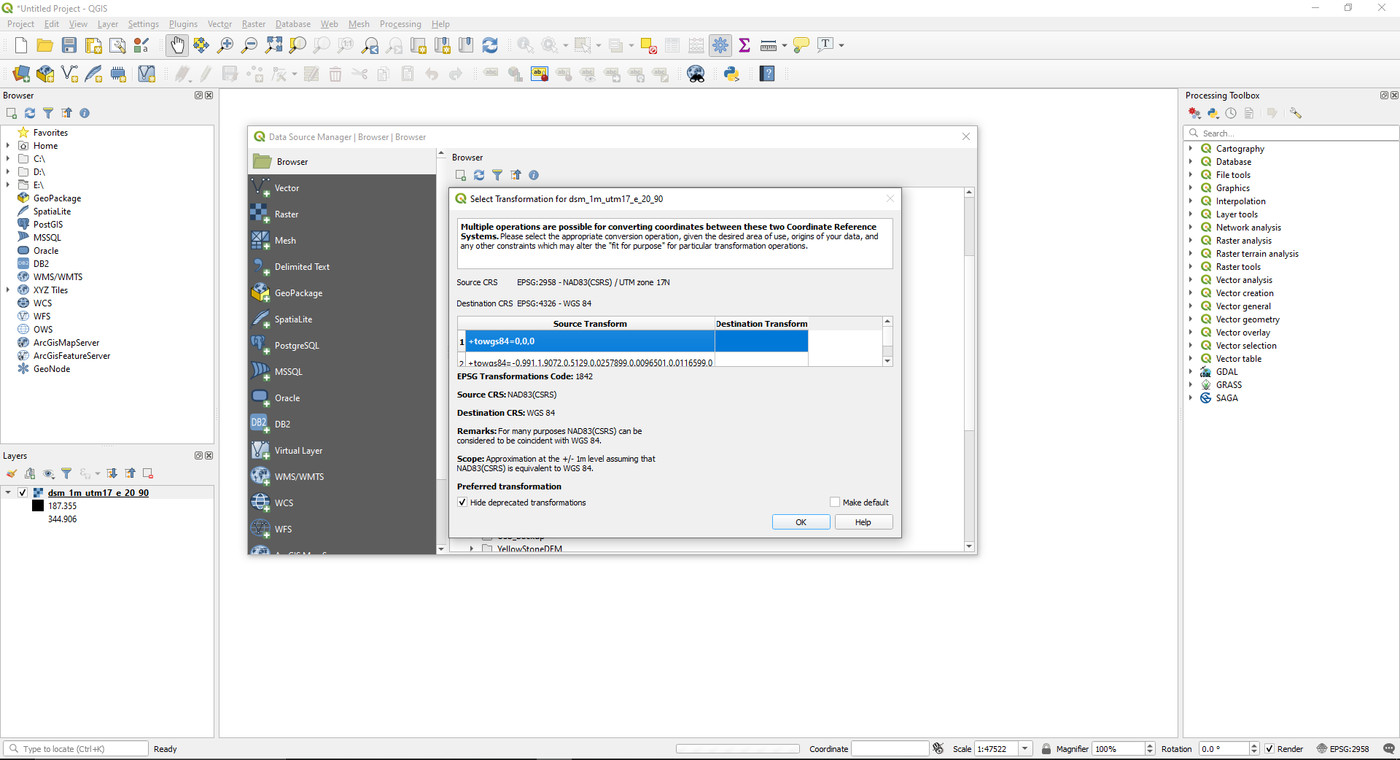
*A popup window will appear when you load in the .tif files, select the first option and click Ok. |
|||
[[File:Import Popup.png|1400px]] |
|||
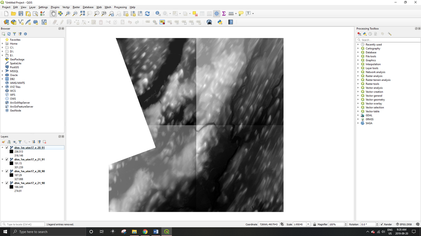
*The result should be the four raster images together in a square, as pictured below: |
*The result should be the four raster images together in a square, as pictured below: |
||
**''Note: If images are too hard to read, clicking on the image twice will result in a larger version of the image.'' |
**''Note: If images are too hard to read, clicking on the image twice will result in a larger version of the image.'' |
||
[[File: |
[[File:Import_Step1.png|1400px]] |
||
===Merging Rasters === |
|||
'''Step 2.''' |
'''Step 2.''' |
||
*Use the merge tool ('''Raster''' -> '''Miscellaneous''' -> '''Merge''') to combine the .tif files into one working |
*Use the merge tool ('''Raster''' -> '''Miscellaneous''' -> '''Merge''') to combine the .tif files into one working raster image. |
||
*In the merge tool, select the four .tif files through the '''Input Layers''' selection, directly under the '''Parameters''' tab. |
*In the merge tool window, select the four .tif files through the '''Input Layers''' selection, directly under the '''Parameters''' tab. |
||
*Under the '''Merged''' heading select the '''Save to File…''' option, give the output a name and save it in your working folder. |
|||
*Once the layers have been selected, click '''Run in Background''' in order to merge the files. |
*Once the layers have been selected, click '''Run in Background''' in order to merge the files. |
||
*The resulting merged file should look similar to the image below: |
*The resulting merged file should look similar to the final image below: |
||
[[File: |
[[File:Merge_Popup_Step2.png|1400px]] |
||
''Using the '''Merge''' tool. |
''Using the '''Merge''' tool. |
||
[[File: |
[[File:Merge_Step2_Example.png|1400px]] |
||
''Merged raster files. |
''Merged raster files. |
||
| Line 72: | Line 101: | ||
'''Step 3.''' |
'''Step 3.''' |
||
* |
*We will now create an '''Area of Interest''' or ('''AOI''') polygon so we can clip our water layers to the boundary of our DTM data in the following step. |
||
*Navigate to '''Layers''' -> '''Create Layer''' -> '''New Shapefile Layer''' |
*Navigate to '''Layers''' -> '''Create Layer''' -> '''New Shapefile Layer''' |
||
*At the top of the window, give a name to your new file ('''AOI''' is suitable), and select '''Polygon''' as the ''Geometry Type'' -> At this point a new layer named '''AOI''' will be created. |
*At the top of the window, give a name to your new file ('''AOI''' is suitable), and select '''Polygon''' as the ''Geometry Type'' -> Click '''OK''', At this point a new layer named '''AOI''' will be created. |
||
*Right click on the newly created '''AOI''' layer, and select '''Toggle Editing.''' Once this is selected, navigate to the top panel and find the '''Add Polygon Feature''' |
*Right click on the newly created '''AOI''' layer, and select '''Toggle Editing.''' Once this is selected, navigate to the top panel and find the '''Add Polygon Feature''' button. [[File:Add_Polygon_Feature_Button.png|32px]] |
||
*Do your best to draw a border around the '''Merged''' layer (hint: ''use your numpad to move your screen when zoomed in''), when complete, right click on the screen and when prompted to save changes to the layer, select '''Yes'''. |
*Do your best to draw a border around the '''Merged''' layer (hint: ''use your numpad to move your screen when zoomed in or click and drag with the scroll wheel to pan''), when complete, right click on the screen and when prompted to save changes to the layer, select '''Yes'''. |
||
* |
*You can now symbolize the polygon with an outline. Right click on the layer and select '''Layer Properties'''/ '''Symbology''' then select '''Outline Red'''. The final '''AOI''' and '''Merged''' layer should look similar to what is shown below: |
||
[[File: |
[[File:CreatingAOI_Step3.png|1400px]] |
||
== |
=== Adding Vector Layers=== |
||
'''Step 4.''' |
'''Step 4.''' |
||
*We can now add the vector Peterborough data to our QGIS session. |
|||
*Once the four raster images have merged, and the AOI has been created around it, the '''City of Ottawa''' files that were downloaded earlier can be added into QGIS. |
|||
*Navigate to the folder they were saved |
*Navigate to the folder they were saved and import each of the shapefiles using the '''Data Source Manager'''. |
||
*Ensure the polygons are overlaying the merged raster layer, and edit the appearance of each feature to your liking (''right click on the layer and select properties to change symbology''). |
|||
*For the purposes of the tutorial, the polygons used were: '''Major Water''', '''Buildings''', '''Roads''', '''Major Roads''', '''Railroads''', and finally '''Bridges'''. |
|||
*Ensure the polygons are overlaying the merged raster layer, and edit the appearance of each feature as you want (''double click on the icon to the left of each layer name''). |
|||
*The resulting file should appear similar to the image presented below: |
*The resulting file should appear similar to the image presented below: |
||
[[File: |
[[File:Vector_Layers_Step4.png|1400px]] |
||
=== Clipping === |
|||
'''Step 5.''' |
'''Step 5.''' |
||
*Now that everything we want is added, the vector layers can be clipped to match the extent of the merged raster layer. |
*Now that everything we want is added, the vector layers can be clipped to match the extent of the merged raster layer. |
||
*Navigate to '''Vector''' -> '''Geoprocessing Tools''' -> '''Clip''' |
*Navigate to '''Vector''' -> '''Geoprocessing Tools''' -> '''Clip''' |
||
*Select the |
*Select the '''Hydrography''' layer as the ''Input Layer,'' and the '''AOI''' as the ''Clip Layer''. This clips the '''Hydrography''' layer to the boundary of the '''AOI''' layer. |
||
*Under the ''Clipped'' section of the popup window select a save location for the output file and change the file type to shapefile (.shp), then click Ok. |
|||
*Repeat this process until all the '''City of Ottawa''' vector layers have been clipped, renaming each newly created layer as ''"name" clip'', or by removing the original layer and reassigning the name to the clipped layer. |
|||
*You can now turn off the original '''Hydrography''' layer or remove it from the session (''right click the layer and select remove''). |
|||
*When all the vector layers have been clipped, the result should look similar to this (remember to symbolize everything that has been clipped): |
|||
[[File: |
[[File:Clipped_Hydrology_Step5.png|1400px]] |
||
===Sink Fill=== |
|||
'''Step 6.''' |
|||
*In this step, the Sink Fill (Wang & Liu) tool will be used from the QGIS toolbox. The tool will sequentially fill any significantly low pixels in the DTM where the flow of water could accumulate incorrectly (''this is generally used to remove sinks from hydrologic analyses''). |
|||
*Navigate to '''Processing''' in the top banner, select '''Toolbox''', this will open a list of available tools. |
|||
*At the bottom of the list select '''SAGA''', look for and select '''Terrain Analysis - Hydrology''' -> '''Fill Sinks (Wang & Liu)'''. The tool window should now open. |
|||
*Under the dropdown list for ''DEM'' select the layer '''Merged''', and select save locations for the three output files ('''Filled DEM''', '''Flow Directions''' and '''Watershed''') then select ''Run''. |
|||
*After the tool has finished, drag the three new layers ('''Filled DEM''', '''Flow Directions''' and '''Watershed''') underneath the vector layers. |
|||
*The final output will look very similar to the image in ''Step 5'', if everything has gone correctly (''if you look closely you may be able to see low points in the DTM that the tool has filled''). |
|||
===Identifying Water level=== |
|||
==Sink Fill== |
|||
'''Step 6.''' |
|||
*In this step, the Sink Fill (Wang & Liu) was used from the QGIS toolbox. This was used in order to fill any spatial outliers that may have an effect on the overall result of the flood risk assessment. |
|||
*Navigate to '''Processing''' at the top of the program, and from there select '''Toolbox''', in order to open the list of available tools. |
|||
*At the bottom of the list of tools is '''SAGA''', select this and continue down until you reach '''Terrain Analysis - Hydrology''' -> '''Fill Sinks (Wang & Liu)''' |
|||
*Under the dropdown list for ''DEM'' select the layer '''Merged''', and select ''Run'' (it's also a good idea to save ''Filled DEM'' to an ''Output'' folder in your primary directory). |
|||
*Upon completion, move your mouse to the ''layers'' area, and move the three new layers ('''Filled DEM''', '''Flow Directions''' and '''Watershed''') underneath the vector layers. |
|||
*The final output will look the same as the image in ''Step 5'', if everything has gone correctly. |
|||
'''Step 7.''' |
|||
*The next step is to determine the current water level of the filled DTM. |
|||
*To do this you will need to install a plugin though the '''Plugins''' tab in the top banner. |
|||
*Click on '''Plugins''' -> '''Manage and Install Plugins''', scroll down until you see the '''Value Tool''', then Click Install Plugin. |
|||
[[File:ValueTool_Plugin.png|1400px]] |
|||
*After installing, close the popup window and you should now see the '''Value Tool''' button on your main taskbar. [[File:ValueTool_Button.png|32px]] |
|||
*By default the tool should be enabled, however if it is not navigate to the '''View''' -> '''Panels''' -> '''Value Tool Panel''' (and make sure the box is checked) |
|||
*Next click on the '''Identify Features''' tool [[File:Identify_Features_Button.png|32px]] on the main toolbar, then click on the '''Value Tool'''. [[File:ValueTool_Button.png|32px]] |
|||
*Zoom in to “Little Lake” in the middle of the downtown Peterborough area. |
|||
[[File:ValueTool_Step7.png|1400px]] |
|||
*You should now see the pixel value of the water surface on your right under the '''Identify Results''' window. |
|||
*You can click around the lake to compare values and see if they change, the Value Tool will continue to select values from the topmost raster image, even if there are polygons over-top. |
|||
*We can now see that the elevation of the water level is approximately 188m. |
|||
===Raster Calculator=== |
=== Raster Calculator=== |
||
'''Step |
'''Step 8.''' |
||
* |
*We will now use the '''Raster Calculator''' tool to establish what areas will be flooded given an increase in water level of 2 meters. |
||
* |
*Under the top banner navigate to '''Raster'''/ '''Raster Calculator'''. |
||
* |
*Recreate the following expression under the '''Raster Calculator Expression''' section of the window: '''( ( "Filled_Merge@1" <=190 ) = 1 ) AND ( ( "Filled_Merge@!" >= 190 ) = 0 )''' |
||
*(Note: the expression will not run properly if you copy and paste it in, you will need write it out manually in the popup window). |
|||
*If entered correctly, ''Expression Valid'' will appear under the expression window, and a new new layer will be created. |
|||
[[File:RasterCalculator_Step.png|600px]] |
|||
*If entered correctly, Expression Valid will appear under the expression window, then select a save location and name for your output file. |
|||
*Click Ok and run the tool. |
|||
*You should end up with an output raster with two values 1 (flooded area, white) and 0 (non-flooded area, black). The output should look like the following image (you may need to rearrange the order of your layers so that the roads, buildings, etc. polygons are on top). |
|||
[[File:RasterCalculator_Flood.png|1400px]] |
|||
=== Changing NoData Values=== |
|||
'''Step 9.''' |
|||
[[File:RasterCalc.PNG|600px]] |
|||
*After creating the raster of the flooded areas, we can now turn this layer into a polygon (with a few intermediate steps). |
|||
*First the 0 value pixels (land) must be turned into no data values. Right click the water raster created in step 8 and click '''Export''' -> '''Save as…''' a popup window should appear. |
|||
*Give the output a file name and save location, then scroll down and check the '''No Data Values''' box. |
|||
*Click on the green plus symbol to add a new value manually, then in the box above type in 0, the left box will autofill to 0 as well, then click OK. |
|||
[[File:SaveAs_Step9.png|1400px]] |
|||
*You should now have a raster of water only areas in black as below. |
|||
==Result== |
|||
[[File:WaterOnly_Step9.png|1400px]] |
|||
=== Raster to Polygon === |
|||
'''Step 6.''' |
|||
*Upon completion of the raster calculator, an output of the ''Ottawa-Gatineau'' downtown area will be given (same extent we have been working with the entire time). |
|||
*The areas that will be flooded given a rise in water levels of ~ 1 meter are in white ('''1'''), while the areas that are untouched remain black ('''0'''). |
|||
**Note: ''The image below has all other layers hidden in order to see the specific area that will be flooded. In order to determine what infrastructure will be affected (and make use of the previous steps), it is important to add all layers back, as seen in the next step.'' |
|||
'''Step 10.''' |
|||
*Go to the top toolbar and click '''Raster''' -> '''Conversion''' -> '''Polygonize (Raster to Vector)…''' |
|||
*Under the '''Input Layers''' heading select the water only raster we created in the previous step. |
|||
*Under the '''Vectorized''' heading select a save location for your output polygon and change the file type to save as a .shp file. |
|||
[[File:Raster_To_Polygon_Step10.png|1400px]] |
|||
*Click OK |
|||
[[File:FirstFlooded.PNG|700px]] |
|||
*The output should be a polygon of the flooded areas as seen below (notice the gap in the raster image on the left has also been included in the new polygon layer, we will need to remove this next) |
|||
[[File:Raster_To_Polygon_Output_Step10.png|1400px]] |
|||
=== Deleting Unwanted Polygons === |
|||
'''Step 11.''' |
|||
*We can now get rid of the no data area that was mistakenly included in our water only polygon. |
|||
*Right click the polygon layer and click '''Toggle Editing'''. |
|||
*In the middle toolbar at the top, click on the '''Select Features by Area or Single Click''' button [[File:SelectFeatures_By_Button.png|32px]], then click on the unwanted polygon. |
|||
*The polygon should now be highlighted in yellow, click the '''Delete Selected''' button [[File:DeleteSelected_Button.png|20px]] to delete the polygon. |
|||
*Right click the polygon layer again and click '''Save Edits''', then '''Toggle Editing''' so that editing is turned off. |
|||
*The unwanted polygon should now be deleted from your flooded area polygon. |
|||
=== Identifying Flooded Buildings === |
|||
'''Step 7''' |
|||
*At this stage the flood analysis is almost complete, but we want to visualize and demonstrate what has been affected by the rising water levels. Simply turn all infrastructure layers back on (i.e. ''Buildings'', ''Roads''). |
|||
*If not visible, move the layers to the top of the ''Layers'' tab/window by dragging them above the layer ''RasterCalcFilled'' (if not renamed). |
|||
*Finally, make adjustments to the symbology (''right-click the layer name'', ''Properties'', ''Symbology'') and use something that demonstrates if the infrastructure is flooded or not, such as an outline. |
|||
*The final output should look similar to the image below: |
|||
'''Step 12.''' |
|||
*We are now able to identify vector objects that are impacted by the flooded areas. |
|||
*To identify all the buildings that have been flooded go to the search bar in the bottom left-hand corner of the screen and type in '''Select by Location''', select the tool form the menu and a popup window should appear. |
|||
*Under the '''Select Features From''' heading select the Building polygon layer, under the '''By Comparing Features From''' heading select your flood water polygon. |
|||
[[File:SelectByLocation_Step12.png|1400px]] |
|||
*Click run. |
|||
*The buildings that intersect with the flooded areas should now be selected and highlighted when you zoom in. |
|||
*Right click the building shapefile and click '''Export''' -> '''Save Selected Features As…''' |
|||
*You can now save all the overlapping features as their own polygon layer. |
|||
*This new layer can then be symbolized differently to highlight what buildings have been flooded. |
|||
*This step can also be repeated with the other vector layers to identify what pedestrian walkways or roads have been flooded. |
|||
[[File:ID_FloodBuildings_Step12.png|1400px]] |
|||
*The tutorial is now complete! |
|||
== References == |
|||
[[File:SecondFloodedPNG.png|700px]] |
|||
<ref>''[https://gisgeography.com/dem-dsm-dtm-differences/ GISGeography]'',''DEM, DSM & DTM Differences – A Look at Elevation Models in GIS'', Last Updated: 2018-02-20, Retrieved: 2019-09-21 </ref> |
|||
Latest revision as of 10:34, 24 October 2019
Contents
Introduction
Flood assessment is one of many practical applications of GIS. This analysis will focus on the city of Peterborough, a small city northeast of Toronto. The analysis is particularly relevant due to past flooding events in the Peterborough area. By a completing flood risk assessments, the city can identify at-risk infrastructure and populations, as well as develop stronger preparedness measures for future flooding events.
The purpose of this tutorial is to provide users with guidance in completing a flood risk assessment, as well as an introductory glance into QGIS.
Software Requirements
In order to begin this tutorial, you will need to download the QGIS software package from the following link (https://www.qgis.org/en/site/ ). This tutorial was created using QGIS version 3.8.1. The latest version of QGIS is freely available for Windows, MacOS X, Linux and Android.
All steps of the tutorial will be completed using this free and open source software, and will not rely on the use of any other programs.
Data
The primary source of data used for this analysis will be the High Resolution Digital Elevation Model (HRDEM) - CanElevation Series, produced by Natural Resources Canada for the city of Peterborough. The dataset is hosted on the Open Data Canada website here: (https://open.canada.ca/data/en/dataset/957782bf-847c-4644-a757-e383c0057995); specific download instructions are provided in the next section, below, but first we'll review different forms of elevation data models.
There are two main types of elevation datasets provided as part of the High Resolution Digital Elevation Model (HRDEM). Both datasets have been derived from airborne LIDAR data.
The two datasets are in the form of a Digital Surface Model (DSM) and a Digital Terrain Model (DTM). It is important to know the difference between these two elevation datasets and how this can affect your analysis of flooded areas.
A Digital Surface Model or DSM is very similar to that of a Digital Elevation Model (DEM) or Digital Terrain Model (DTM). All three show elevation data of the earth’s surface relative to sea level. One major distinction between a DSM and a DTM is the presence of man-made and natural features. The DSM shows the tops of buildings, houses, highways, tree canopies, vegetated surfaces and all manor of other solid features above the surface of the ground. They are traditionally in the form of a raster image. DSM’s are generally used for purposes where it is necessary to see objects protruding from the surface of the earth. This includes tasks such as assessing the encroachment of vegetation or viewshed analysis for a new High-rise [1]
. They are not used for hydrologic modelling such as a flood analysis.
A Digital Elevation Model or DEM does not include features that protrude from the ground. A DEM represents the ground elevation from sea level. Therefore, the tops of trees, buildings and other features have been removed to reveal the ground underneath. This is very useful for the purpose of hydrologic mapping, such as flood analysis. DEM’s are generally in the form of a raster image [2].
A Digital Terrain Model or DTM can have varying definitions. In some cases, Digital Terrain Model and Digital Elevation Model are used interchangeably. This means that the DTM dataset would be a raster image of the Earth’s surface excluding buildings and vegetation. In other cases, a Digital Terrain Model can be essentially a DEM represented through point data. The dataset shows the elevation of the earth’s surface through a series of equally spaced points (although, in older datasets these points can be unevenly spaced). These points have an associated x and y value along with a third value for elevation. In this case the DTM would be in the form of a vector dataset, such as a shapefile [3].
The DTM dataset available through the High Resolution Digital Elevation Model link is in the form of a geotiff (.tif). This means it is essentially the same as a DEM and can be used for our flood mapping analysis. The DTM data that we will be using in this analysis will be at a resolution of 1m and will be projected in the UTM NAD83 (CSRS) coordinate system.
Additional vector data will also be used in this analysis from the Peterborough Open Data Hub. This includes building footprints, roads, pedestrian footpaths and hydrography polygons.
- See next section for instructions on how to download the files.
Downloads
- Peterborough Digital Terrain Model Data
- High Resolution Digital Elevation Model (HRDEM) - CanElevation Series
- The High Resolution Digital Elevation Model (HRDEM) - CanElevation Series dataset hosted on the Open Canada Data web portal, where you can download different sets of DTM and DSM data across Canada
- 1. Click on the following link. This will take you to the directory where all of the DTM data is stored for the UTM 17 Zone.
- 2. Use the find function (Ctrl + F) to find each of the three images listed below in the file directory.
- 1m_utm17_e_20_90
- 1m_utm17_e_21_90
- 1m_utm17_e_21_91
- 3. Download each file into a folder on your computer. This will be a working folder for all of your flood analysis data.
- Peterborough Vector Data
- This data is hosted by Peterborough's GIS Open Data initiative on their Open Data web portal.
- 1. Click on the following links and download the data as .shp files (a .zip file will be downloaded)
- Hydrography Polygons: This is a polygon of all the waterways in Peterborough.
- Buildings: This is a polygon layer of all the building footprints in Peterborough.
- Roads: This is a line layer of all the road networks in Peterborough.
- Pedestrian Network Polygon: This is a polygon layer of all the pedestrian footpaths and bike trails in Peterborough.
- 2. Go to the .zip files you previously downloaded and extract them to the same folder as you Peterborough DTM data.
QGIS Methods and Instructions
Importing and Merging
Step 1.
- Open Qgis.
- Upload the .tif DTM images in QGIS by clicking on the Data Source Manager button
 . The Data Source Manager window will then appear.
 - Select the folder where your files are saved, (this folder can be added to your favourites by right clicking the folder and adding it to your favourites) drag in all four .tif files to the main window (ignore the .tif.ovr files and only use the .tif files). Alternatively, you can double click each file separately to add them to the project one by one.
- A popup window will appear when you load in the .tif files, select the first option and click Ok.
- The result should be the four raster images together in a square, as pictured below:
- Note: If images are too hard to read, clicking on the image twice will result in a larger version of the image.
Merging Rasters
Step 2.
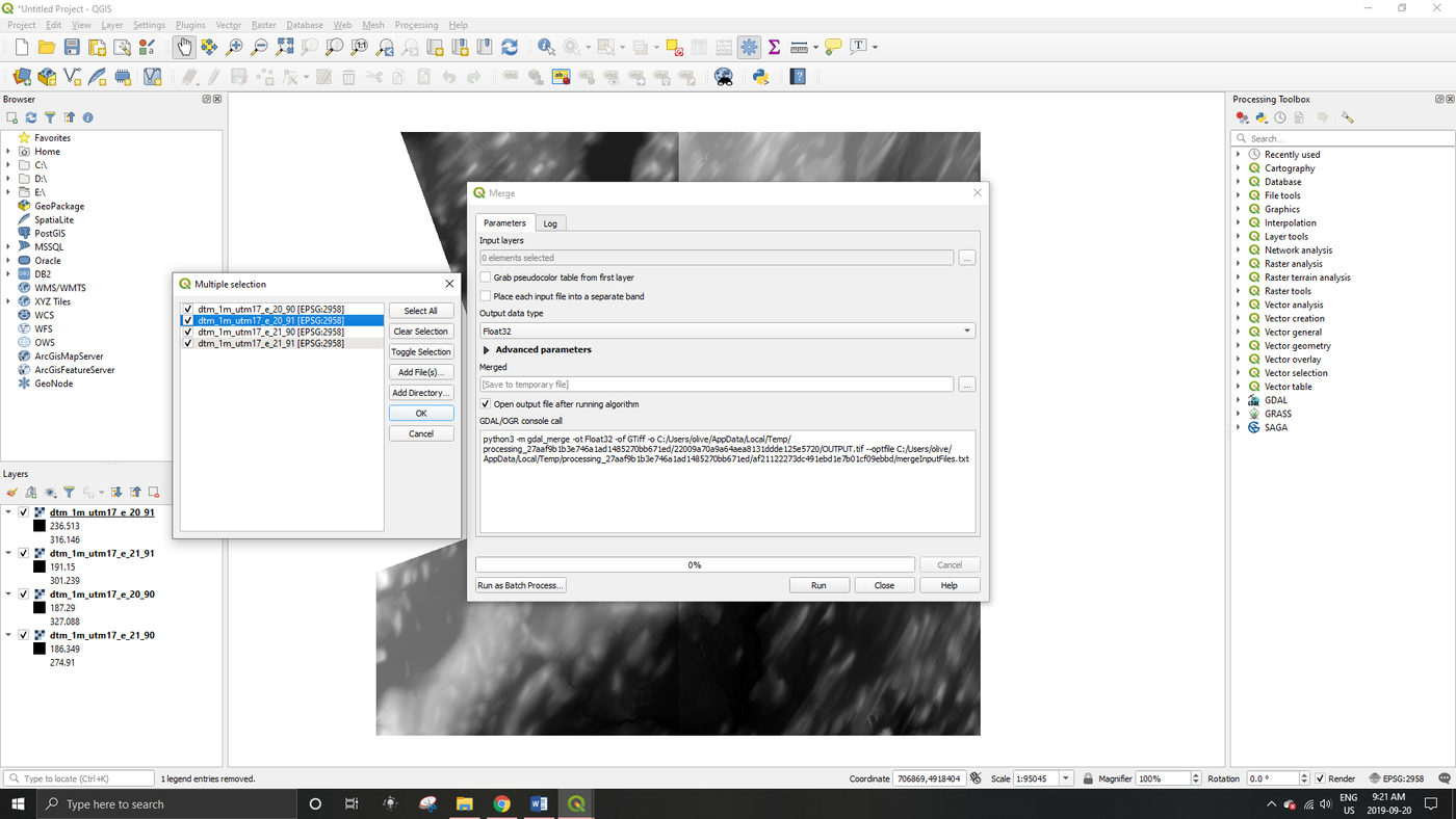
- Use the merge tool (Raster -> Miscellaneous -> Merge) to combine the .tif files into one working raster image.
- In the merge tool window, select the four .tif files through the Input Layers selection, directly under the Parameters tab.
- Under the Merged heading select the Save to File… option, give the output a name and save it in your working folder.
- Once the layers have been selected, click Run in Background in order to merge the files.
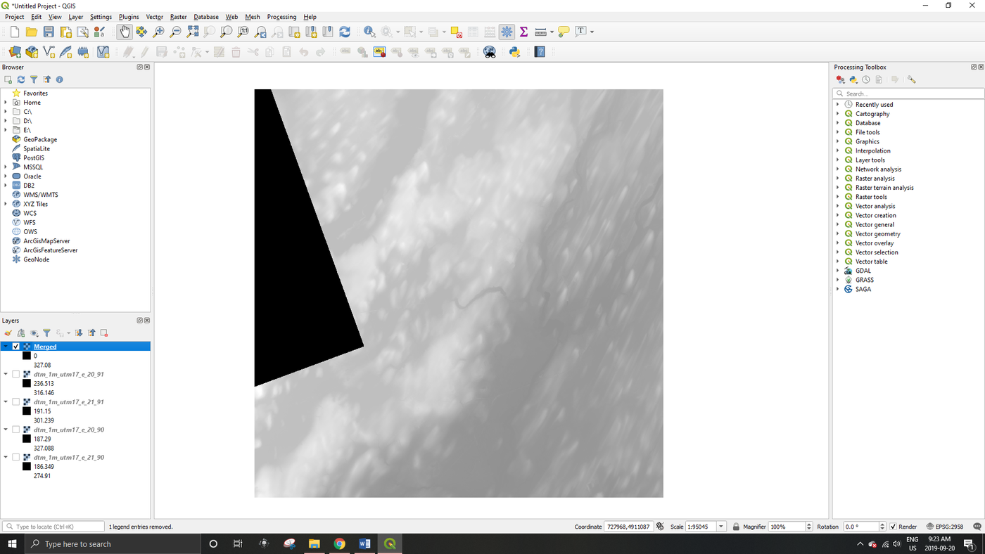
- The resulting merged file should look similar to the final image below:
Creating an AOI
Step 3.
- We will now create an Area of Interest or (AOI) polygon so we can clip our water layers to the boundary of our DTM data in the following step.
- Navigate to Layers -> Create Layer -> New Shapefile Layer
- At the top of the window, give a name to your new file (AOI is suitable), and select Polygon as the Geometry Type -> Click OK, At this point a new layer named AOI will be created.
- Right click on the newly created AOI layer, and select Toggle Editing. Once this is selected, navigate to the top panel and find the Add Polygon Feature button.

- Do your best to draw a border around the Merged layer (hint: use your numpad to move your screen when zoomed in or click and drag with the scroll wheel to pan), when complete, right click on the screen and when prompted to save changes to the layer, select Yes.
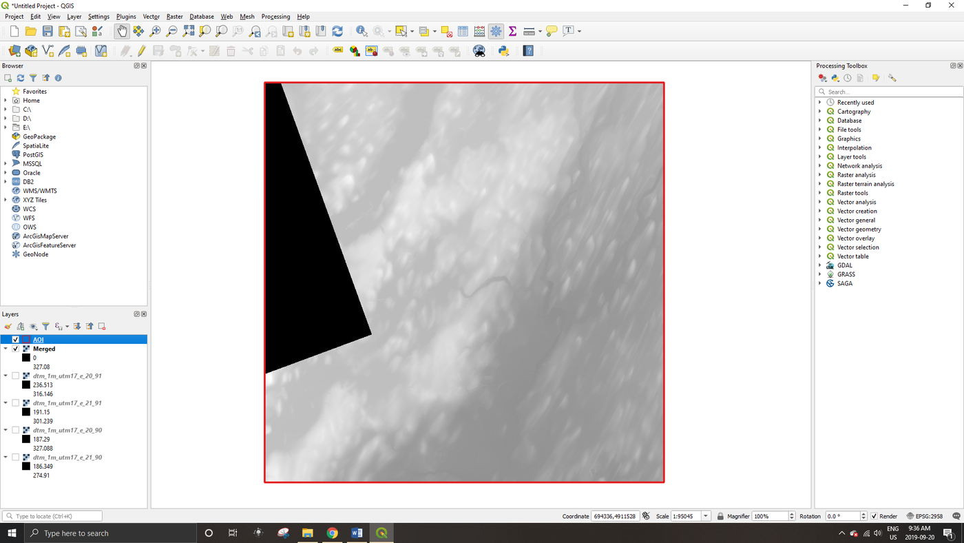
- You can now symbolize the polygon with an outline. Right click on the layer and select Layer Properties/ Symbology then select Outline Red. The final AOI and Merged layer should look similar to what is shown below:
Adding Vector Layers
Step 4.
- We can now add the vector Peterborough data to our QGIS session.
- Navigate to the folder they were saved and import each of the shapefiles using the Data Source Manager.
- Ensure the polygons are overlaying the merged raster layer, and edit the appearance of each feature to your liking (right click on the layer and select properties to change symbology).
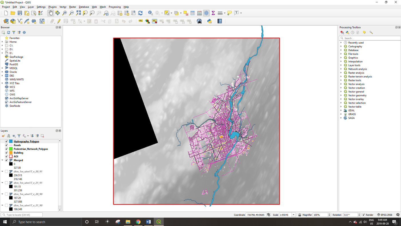
- The resulting file should appear similar to the image presented below:
Clipping
Step 5.
- Now that everything we want is added, the vector layers can be clipped to match the extent of the merged raster layer.
- Navigate to Vector -> Geoprocessing Tools -> Clip
- Select the Hydrography layer as the Input Layer, and the AOI as the Clip Layer. This clips the Hydrography layer to the boundary of the AOI layer.
- Under the Clipped section of the popup window select a save location for the output file and change the file type to shapefile (.shp), then click Ok.
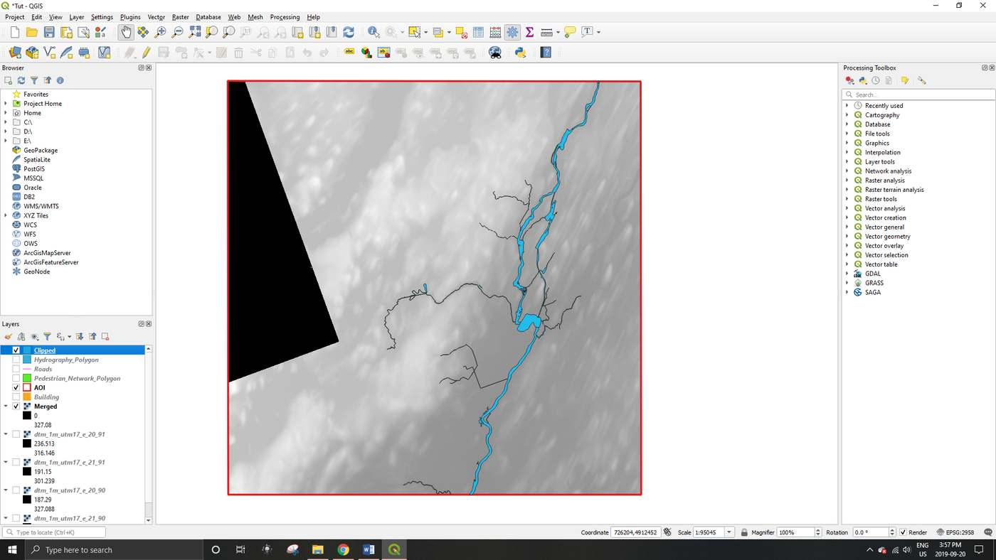
- You can now turn off the original Hydrography layer or remove it from the session (right click the layer and select remove).
Sink Fill
Step 6.
- In this step, the Sink Fill (Wang & Liu) tool will be used from the QGIS toolbox. The tool will sequentially fill any significantly low pixels in the DTM where the flow of water could accumulate incorrectly (this is generally used to remove sinks from hydrologic analyses).
- Navigate to Processing in the top banner, select Toolbox, this will open a list of available tools.
- At the bottom of the list select SAGA, look for and select Terrain Analysis - Hydrology -> Fill Sinks (Wang & Liu). The tool window should now open.
- Under the dropdown list for DEM select the layer Merged, and select save locations for the three output files (Filled DEM, Flow Directions and Watershed) then select Run.
- After the tool has finished, drag the three new layers (Filled DEM, Flow Directions and Watershed) underneath the vector layers.
- The final output will look very similar to the image in Step 5, if everything has gone correctly (if you look closely you may be able to see low points in the DTM that the tool has filled).
Identifying Water level
Step 7.
- The next step is to determine the current water level of the filled DTM.
- To do this you will need to install a plugin though the Plugins tab in the top banner.
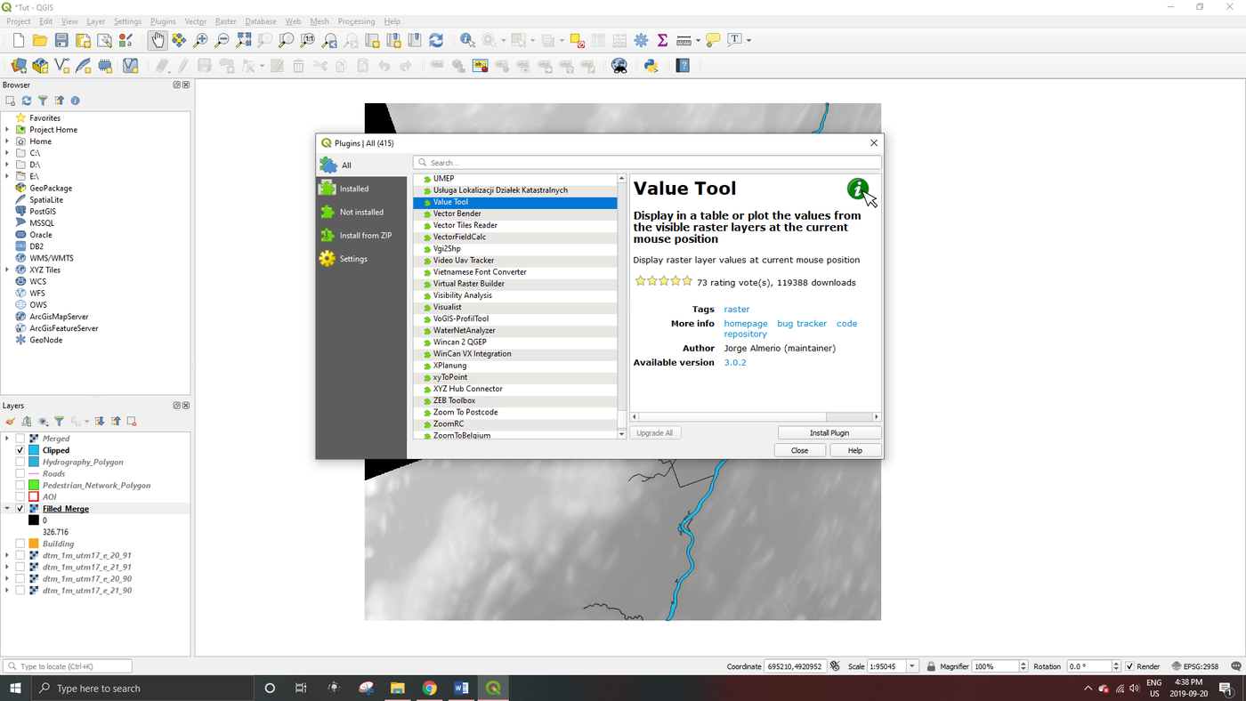
- Click on Plugins -> Manage and Install Plugins, scroll down until you see the Value Tool, then Click Install Plugin.
- After installing, close the popup window and you should now see the Value Tool button on your main taskbar.

- By default the tool should be enabled, however if it is not navigate to the View -> Panels -> Value Tool Panel (and make sure the box is checked)
- Next click on the Identify Features tool
 on the main toolbar, then click on the Value Tool.
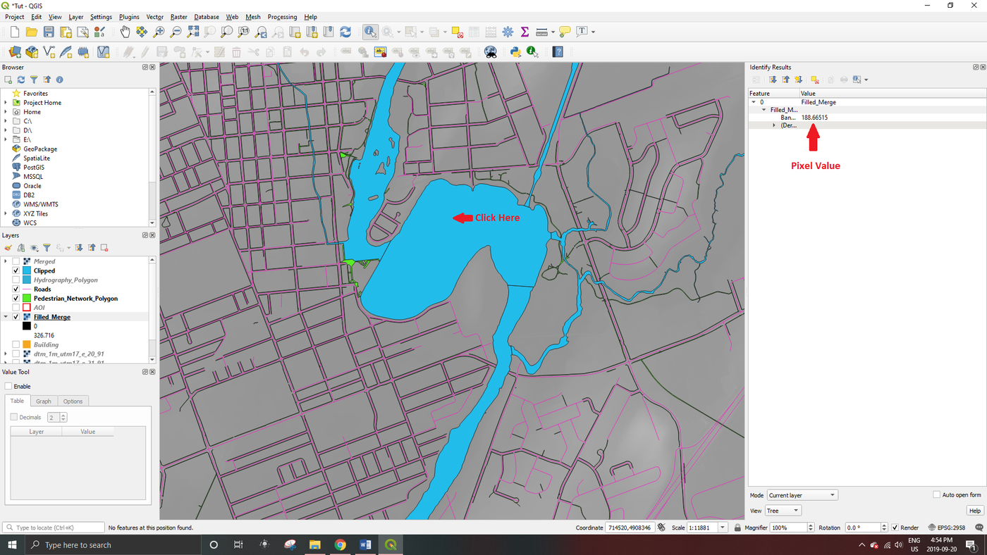
- Zoom in to “Little Lake” in the middle of the downtown Peterborough area.
- You should now see the pixel value of the water surface on your right under the Identify Results window.
- You can click around the lake to compare values and see if they change, the Value Tool will continue to select values from the topmost raster image, even if there are polygons over-top.
- We can now see that the elevation of the water level is approximately 188m.
Raster Calculator
Step 8.
- We will now use the Raster Calculator tool to establish what areas will be flooded given an increase in water level of 2 meters.
- Under the top banner navigate to Raster/ Raster Calculator.
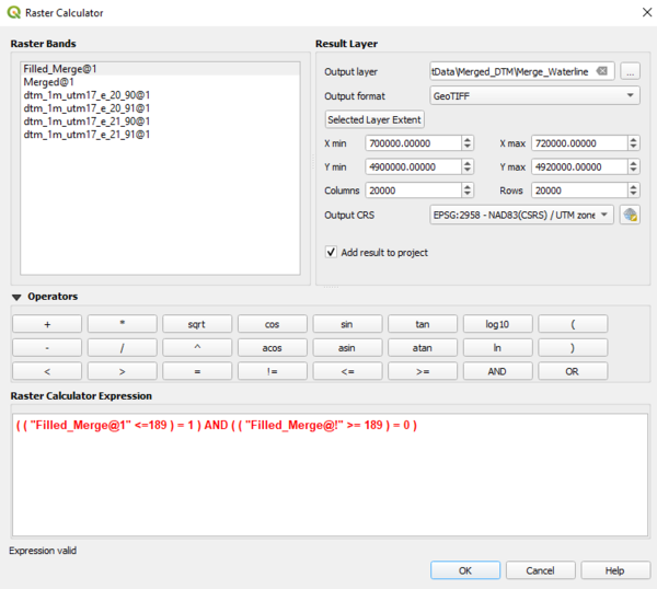
- Recreate the following expression under the Raster Calculator Expression section of the window: ( ( "Filled_Merge@1" <=190 ) = 1 ) AND ( ( "Filled_Merge@!" >= 190 ) = 0 )
- (Note: the expression will not run properly if you copy and paste it in, you will need write it out manually in the popup window).
- If entered correctly, Expression Valid will appear under the expression window, then select a save location and name for your output file.
- Click Ok and run the tool.
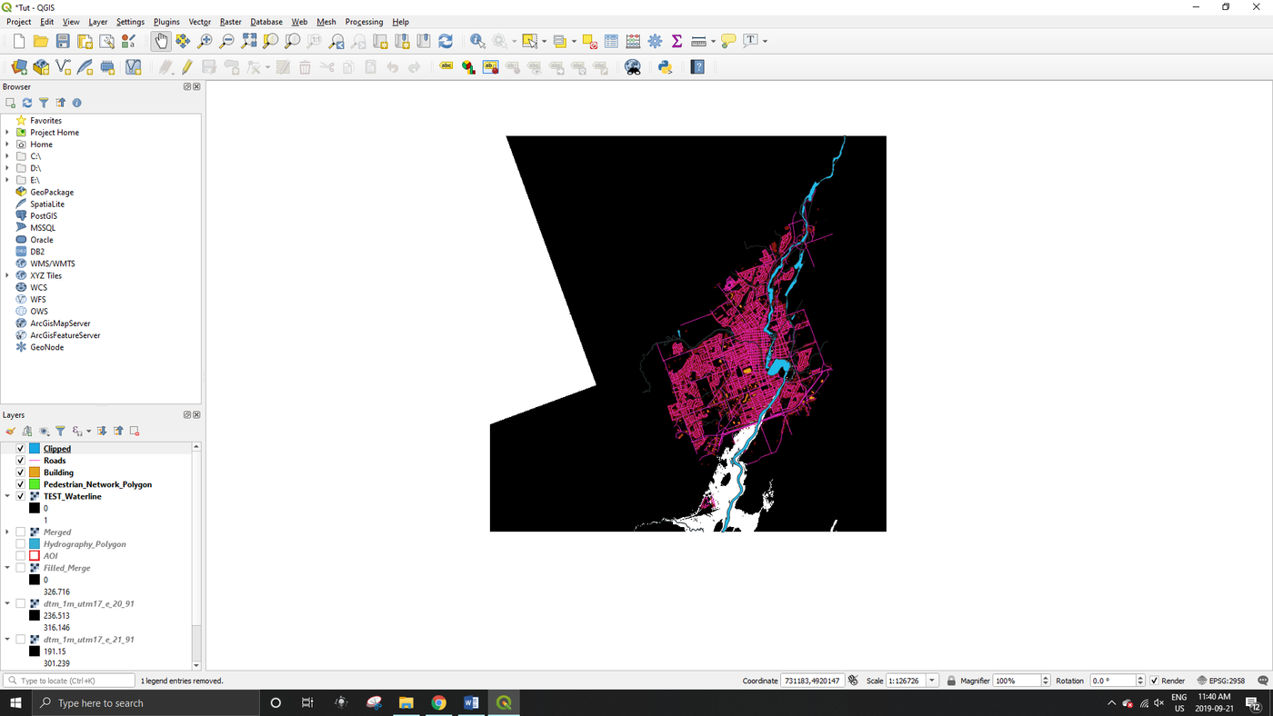
- You should end up with an output raster with two values 1 (flooded area, white) and 0 (non-flooded area, black). The output should look like the following image (you may need to rearrange the order of your layers so that the roads, buildings, etc. polygons are on top).
Changing NoData Values
Step 9.
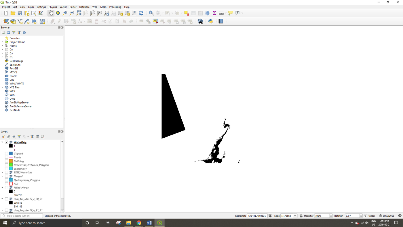
- After creating the raster of the flooded areas, we can now turn this layer into a polygon (with a few intermediate steps).
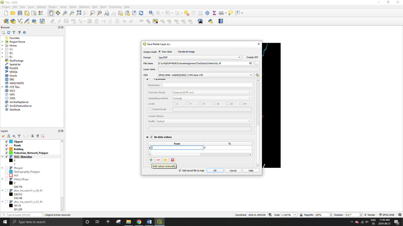
- First the 0 value pixels (land) must be turned into no data values. Right click the water raster created in step 8 and click Export -> Save as… a popup window should appear.
- Give the output a file name and save location, then scroll down and check the No Data Values box.
- Click on the green plus symbol to add a new value manually, then in the box above type in 0, the left box will autofill to 0 as well, then click OK.
- You should now have a raster of water only areas in black as below.
Raster to Polygon
Step 10.
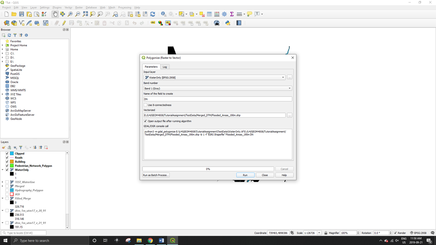
- Go to the top toolbar and click Raster -> Conversion -> Polygonize (Raster to Vector)…
- Under the Input Layers heading select the water only raster we created in the previous step.
- Under the Vectorized heading select a save location for your output polygon and change the file type to save as a .shp file.
- Click OK
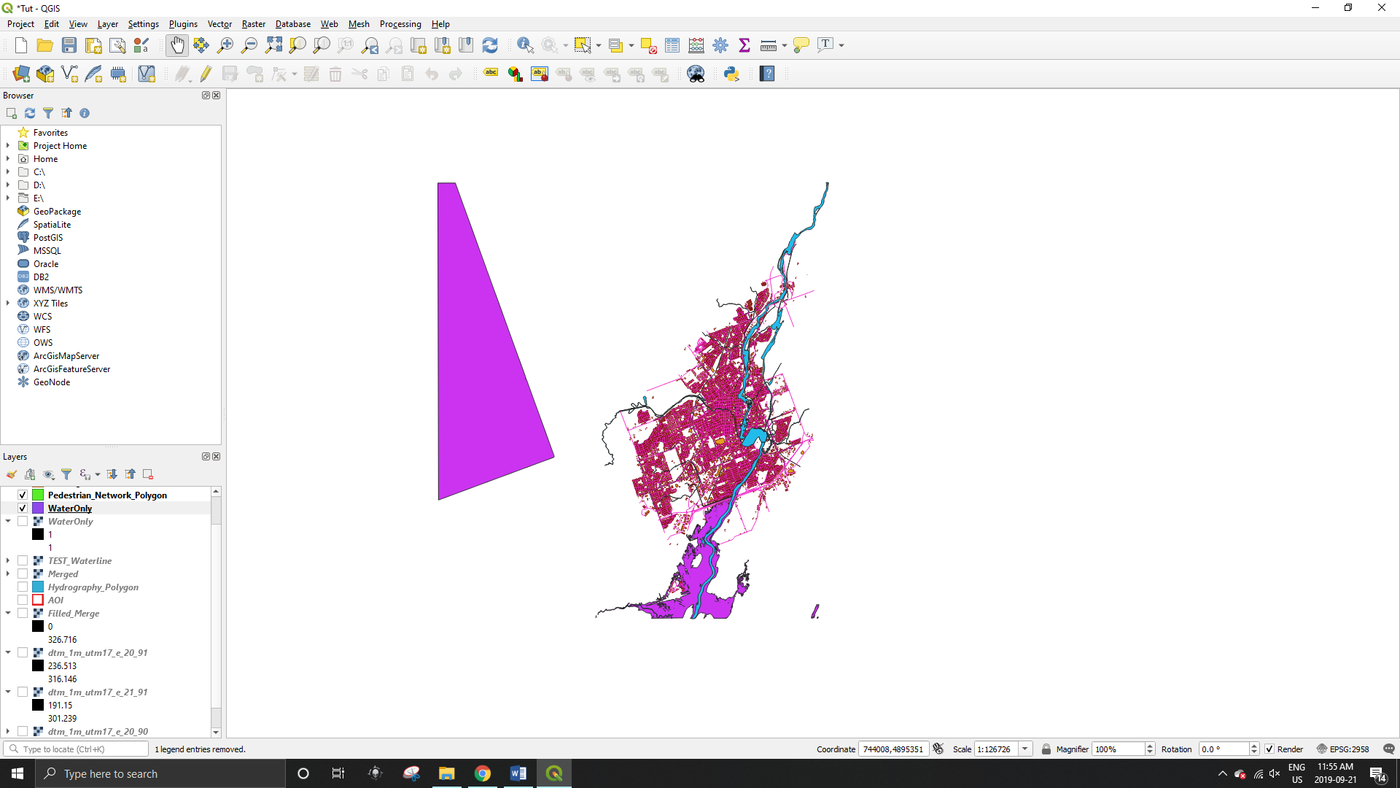
- The output should be a polygon of the flooded areas as seen below (notice the gap in the raster image on the left has also been included in the new polygon layer, we will need to remove this next)
Deleting Unwanted Polygons
Step 11.
- We can now get rid of the no data area that was mistakenly included in our water only polygon.
- Right click the polygon layer and click Toggle Editing.
- In the middle toolbar at the top, click on the Select Features by Area or Single Click button
 , then click on the unwanted polygon.
 - The polygon should now be highlighted in yellow, click the Delete Selected button
 to delete the polygon.
 - Right click the polygon layer again and click Save Edits, then Toggle Editing so that editing is turned off.
- The unwanted polygon should now be deleted from your flooded area polygon.
Identifying Flooded Buildings
Step 12.
- We are now able to identify vector objects that are impacted by the flooded areas.
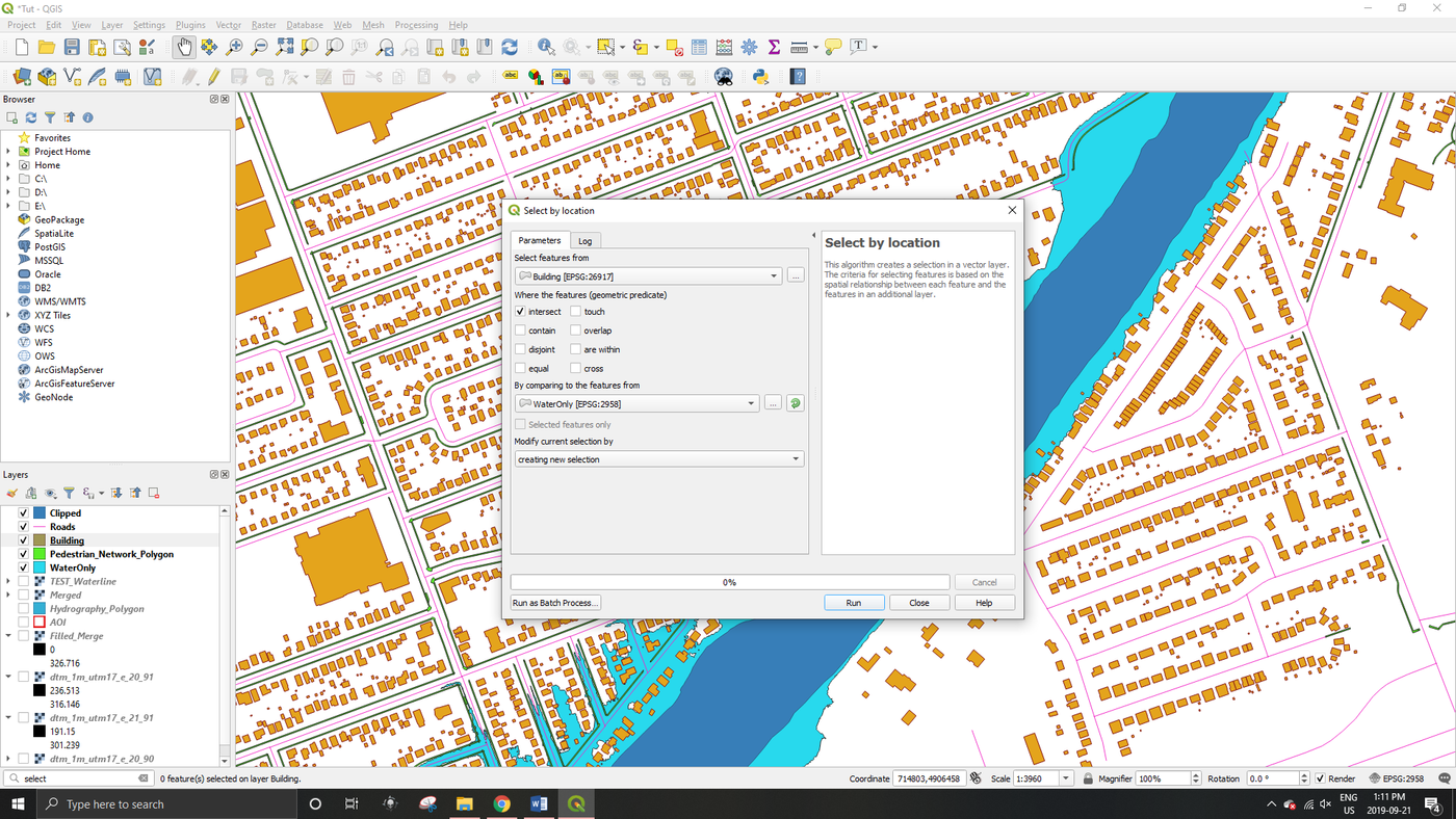
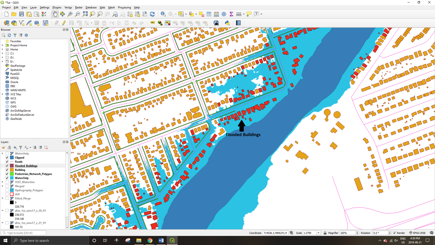
- To identify all the buildings that have been flooded go to the search bar in the bottom left-hand corner of the screen and type in Select by Location, select the tool form the menu and a popup window should appear.
- Under the Select Features From heading select the Building polygon layer, under the By Comparing Features From heading select your flood water polygon.
- Click run.
- The buildings that intersect with the flooded areas should now be selected and highlighted when you zoom in.
- Right click the building shapefile and click Export -> Save Selected Features As…
- You can now save all the overlapping features as their own polygon layer.
- This new layer can then be symbolized differently to highlight what buildings have been flooded.
- This step can also be repeated with the other vector layers to identify what pedestrian walkways or roads have been flooded.
- The tutorial is now complete!
References
- ↑ GISGeography,Retrieved: 2019-09-21
- ↑ GISGeography,Retrieved: 2019-09-21
- ↑ GISGeography,Retrieved: 2019-09-21
- ↑ GISGeography,DEM, DSM & DTM Differences – A Look at Elevation Models in GIS, Last Updated: 2018-02-20, Retrieved: 2019-09-21
