Hazardous Areas Around Linear Infrastructure

Introduction =

Introduction Mountainous terrain can pose challenges for linear infrastructure such as railway lines and highways. Not only do such areas present operational challenges, they also pose risks due to landslides, rockslides, and avalanches that can lead to physical damage, temporary closure, and even loss of life. Having information on potential locations for landslides and rockslides can be helpful in taking preventitive action to reduce risks. Locations can be derived by examining the conditions that can make an area prone to such an event. Such conditions can include the landscape slope, soil type, rock type, precipitation levels, and land use.

This tutorial will focus on railway infrastructure. It will do an analysis of a railway line in Western Austria known as the Vorarlberg Bahn that runs from Bludenz to Bregenz, the capital of Voralberg Land, with a connection to Switzerland. The line is a continuation of the Arlberg Bahn that runs from Innsbruck to Bludenz. It is 68 kilometres long and runs through the Walgau and Rhine valleys. It is owned and operated by the Austrian Federal Railways.

Objective

The objective of this analysis is to find locations along a section of railway infrastructure that are hazardous in that they could be areas prone to landslides or rockslides.

Methods

Data Used

Data Sources Data for this analysis came from various open data sources. A project folder should be set up for the project (e.g. titled RailInfrastruture) and the data downloaded and unzipped into this folder.

• A map of the Austrian rail network can be found on the following GIS data site:

Austria railway network: https://mapcruzin.com/free-austria-arcgis-maps-shapefiles.htm

• A political map of Vorarlberg Land used to clip Austria wide vector and raster files was obtained from Land Vorarlberg:

http://data.vorarlberg.gv.at/ogd/basisdaten/politische_gemeindegrenze.shtm

• An annual rainfall shapefile for Vorarlberg was obtained from Land Vorarlberg:

http://data.vorarlberg.gv.at/ogd/geographieundplanung/jaehrliche_niederschlagss.shtm

• A DEM raster file for Austria was obtained from the Government of Austria through Open Data Osterreich:

https://www.data.gv.at/katalog/dataset/b5de6975-417b-4320-afdb-eb2a9e2a1dbf Click on “zur Ressource” to obtain file.

• A geology shapefile of Austria was obtained from the Geological Survey of Austria (GBA):

https://www.geologie.ac.at/en/produkte-shop/geodaten-software/bersichtskarten/

• A soil shapefile of Austria Austrian Research Centre for Forests (BFW):

https://bfw.ac.at/rz/bfwcms2.web?dok=8548

• A landcover/land use raster file of Europe was obtained from the Copernicus Land Monitoring Service:

CLC_2018 Map https://land.copernicus.eu/pan-european/corine-land-cover Please note that you have to register to access the data, but registration is free.

Software Used

The exercises demonstrated are completed using the Quantum GIS 3.8.1 Zanzibar software interface. These are open source software materials which are freely accessible and available online. For new users it is suggested to use the standalone installer.

This is available by clicking this hyperlink. Click this!

Starting Map Project

The first step is to open QGIS and load all of the shapefiles and raster files into a new project. Vector files are added by selecting “Layer” on the top menu, then add “Add Layer”, and then “Add Vector Layer”. For the Raster Files, the procedure is similar, but “Add Raster Layer” is selected.

File Projections

The map projection used for this analysis was EPSG:31254-MGI/Austria GK West.

The initial file projections were as follows:

• Austrian rail network shapefile: EPSG:4326 -WGS 84
• Political shapefile of Vorarlberg: EPSG:31254 MGI/Austria GK West
• Annual rainfall shapefile: 31254 MGI/Austria GK West
• DEM Raster file:USER Generated CRS
• Geology shapefile: 31287 – MGI Austria Lambert
• Soil shapefile: EPSG:3035 – ETR89
• Land cover/land use raster file: EPSG:3035 -ETRS89/LAEA Europe

The second step is to re-project the data. The following files had to be re-projected: Austrian rail network (vector), DEM (Raster), Geology (Vector), soil (Vector), and land cover/land use (Raster).

Reprojection of Vector Files

To re-project the two vector files, select “Vector” from the top menu, then “Data Management Tools” and “Reproject Layer”. On the “Reproject Layer” window, select the layer to be re-projected as the “Input Layer” and the “Target CRS” as EPSG:31254-MGI/Austria GK West. The “Reprojected” box is used to setup the file for the re-projected layer. Press the “…” button, select “Save to File’, select the project folder and a file name for the re-projected file. The image below shows the “Reproject Layer” window for the vector files that need to be re-projected:

Re-projection Window

Clipping Vector Files to Area of Interest

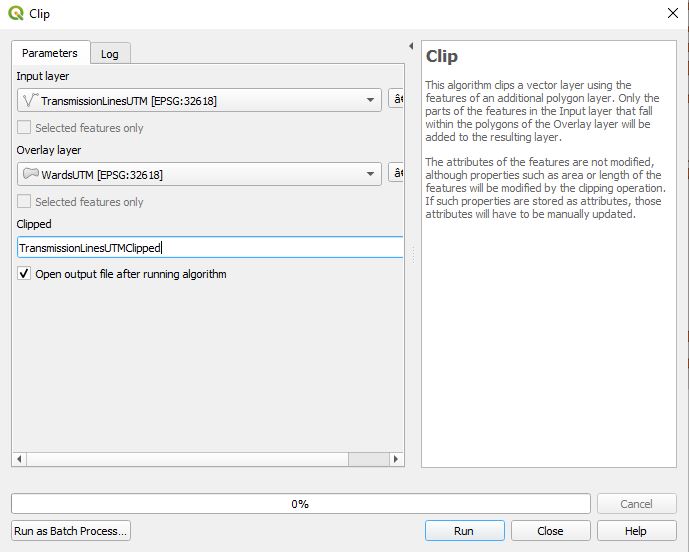
The next step is to clip the vector files to the area of interest, Vorarlberg Land. The Annual Rainfall shapefile is already for Vorarlberg, so the “Railways”, “Geology” and “Soils” shapefiles need to be clipped. To clip these vector files, select “Vector” from the top menu, then “Geoprocessing Tools”, then “Clip”. For the “Input layer”, select the file to be clipped (Railway Reprojected, SoilsReprojected or GeologyReprojected), then select the area of interest, Vorarlberg Political Map, as the “Overlay layer”. Under “Clipped”, select the “…” button, move to the folder where the project files are stored, and enter a name for the new layer under “File name” and press “Save”. This must be done for the three vectors to be clipped.

Clip Window

The Resulting Layers:

1. Next the vector files must be clipped to fit within the extent of the Ottawa area. If all your data fit within the boundaries of Ottawa, skip this step.
   1. Select the 'Vector' tab at the top, the 'Geoprocessing' menu and select the Clip tool.
   2. In the 'Input layer' section select the layers that need to be clipped down. Do this individually for each layer that needs to be clipped.
   3. In the 'Clip layer' section select the layer that will act as your extent, the Wards layer.
   4. The next section is for specifying your output. Click the 3-dot button and and select save to file. Name your new file with details (example: TransmissionLinesUTMClipped), and save click save in that new window.
   5. Make sure the box under the output section is checked to allow the program to automatically add it to your working layers.
2. If the clipping tool has a blank output and you get a warning message that the CRS do not align and will cause problems, this is the solution to that problem (skip if the clipping worked):
   1. Click the CRS button on the bottom toolbar of the program, beside the speech bubble. At the top of that popup, you want to enable the 'On the fly' transformation, if it is not enabled already.
   2. From here, select the layer in the Layers Panel that is not aligning with your desired CRS, and right click it. From this menu select the 'save as' option and create the same shapefile with a new name, and with the CRS of the project. This creates the shapefile again, but this time with the CRS aligning with the project, and allowing you to work with the layers using geoprocessing tools.
3. If your layer has a geometry error that prevents clipping (the Water and Wooden Area layer has this problem), the solution to this problem is to create a buffer for the layer with a value of zero. This can be accomplished by selecting the "Vector" from the top menu, the "Geoprocessing" tools from the drop down menu, and then selecting "Buffer". For the input layer, select the layer with the geometry problem that needs to be buffered, and set the Distance at 0 metres. Under "Buffered", click the 3-dot button and and select save to file. Name your new file with details (example: WaterZeroBuffer) and click "Run" in that new window. The buffered layer should then appear in your layer list. It should be renamed accordingly by right clicking on the layer, selecting properties, selecting "source" from the side menu, and changing the layer name in the "Layer Name" box.

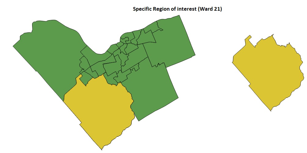
Narrowing Results to a Specific Delineation Area

This section focuses on narrowing the view to a specific area of interest. In this case the area of interest is Ward 21, Rideau-Goulbourn. This is a largely rural/agricultural ward of the city, making it a prospective optimal area for the production of wind energy. This process will involve the exporting of the specified area as a new shapefile.

1. The following steps demonstrate the exportation of a specific area of interest as a new shapefile:
   1. Right click the "Wards" layer in the layer panel, and select the " Attribute Table".
   2. Next, select the ward you want to create a new shapefile out of, this time being ward 21.
   3. Close the attribute table and then select the "Save as" option from the Layer drop-down menu located at the top. Select "ESRI Shapefile" from the "Format" dropdown menu, enter the filename, and then check the projection through the CRS drop down menu. The recommended CRS is WGS84/UTM Zone 18N EPSG 32618. Under "Encoding", check-off "Save only selected features" Press okay.
   4. Add the newly created shapefile to the map project if not already present.
2. With the new ward extent shapefile, you want to trim the extra data down to fit within it.
   1. It is similar to the clipping tool, but this time select the 'Intersection' tool.
   2. Input the data you want to cut down and show them instead of the full extent shapefiles.

Visualization of Restrictions using a Buffer

This section will demonstrate how to add a buffer region to each of the vector layers representing the limitations imposed by the spatial restrictions set by the Government of Ontario.

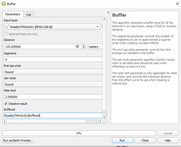
1. Open the "Vector" tab and go to the "Geoprocessing" menu, and select the "Buffer" tool
2. To create the railway buffer, select the Railway Lines layer under the 'Input layer' field
   1. Set the 'Distance' field to 135 (this number represents the 135m restriction applied to Railways)
   2. Leave 'Segment' as the default 5, as changing this does not have a significant impact on the end result.
   3. Make sure the dissolve box is checked, which makes the buffer a continuous shape, instead of separate entities.
   4. Click the 3-dot button and and select save to file, name your new file with details (example: RailwayLinesUTMClippedBuffer135m), and click save in that new window.
   5. Click Run, and wait for the output to successfully finish (this may take an extended period of time depending on the size of the input vector layer
3. 
4. Complete this process for Road Layers, again setting the 'Distance' to 135 as the restriction for roads is the same as railways.
5. When completing this process for the Transmission Lines layer, make sure to change the 'Distance' parameter to 1000 to meet the 1000m restriction imposed on this infrastructure.
6. For both "Water" and "Wooded Area", make sure to change the "Distance" parameter to 120 metres to meet the 120 m restriction imposed on these areas.

Representation of the Resulting Layers:

Creation of Total Suitable Areas Using an Overlay

This section will demonstrate the use of vector overlay techniques in order to visualize the suitable areas for wind turbines that are free of spatial restrictions.

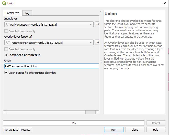
Using Union to Create a Merged Buffer Layer

1. Select the 'Vector' tab, select 'Geoprocessing tools' and select 'Union' as the last part of the menu.
   1. Under the 'input layer' field choose the Railway Buffer layer.
   2. Under the 'input layer 2' field choose the Transmission Lines Buffer layer.
   3. Under the 'Union' field provide an output name (example: RailwayTransmissionLinesUnion)
   4. Click run, and wait for the output to successfully finish.
2. Return to the 'Union' tool.
   1. Under the 'Input layer' field choose the Union layer just created (example: RailwayTransmissionLinesUnion).
   2. Under the 'Input layer 2' field choose the Roads Buffer layer.
   3. Under the 'Union' field provide an output name (example: RailwayTransmissionLinesRoadsUnion)
   4. Click run, and wait for the output to successfully finish.
   5. Repeat the same process for Water and Wooded Area to add these two buffered areas to the "Union" layer thus creating two more union layers (RailwayTransmissionLinesRoadsWaterUnion and RailwayTransmissionLinesRoadsWaterWoodedAreaUnion). The latter layer is the final merge layer incorporating all five buffers.

Using Dissolve to Clean Up the Final Merged Buffer Layer

1. Return to the 'Geoprocessing tools' tab and select the tool 'Dissolve'. This will clean up the merged layers.
   1. Select the shapefile you just created as the final merge, and check the box 'Dissolve All'.

This process results in the overlay of all five buffer restriction layers providing a total suitability layer which considers all restrictions.

Representation of the Resulting Layer:

Identifying Largest Suitable Area

The Largest suitable area can be identified using the 'measurement tool' located on the toolbar. However, this would take a lot of time to outline each shape, so I will show you a way to calculate each area.

1. The first step is to go 'Vector'>'Geoprocessing'> 'Difference'.
   1. Select the extent area as the input and the merged buffers as the difference.
2. You now can see each individual shape away from the buffers, which allows us to calculate the area of each shape.
   1. First we must separate them in the attribute table, and to do this we must create another shapefile. To do this go 'Vector'>'Geometry'> 'Multiparts to Singleparts'.
   2. Select the created shapefile from the 'Difference' tool and create a new shapefile of separated features.
3. Now turn on editing of this new shapefile, and open the attribute table to reveal the large number of features present in this shapefile.
   1. You can turn on editing by right-clicking the layer in the Layer Panel and selecting the 'Toggle Editing' option.
   2. Once in the attribute table create a new field. You will want to name the field "area" and select 'Decimal Number'. Precision and Length can be left default.
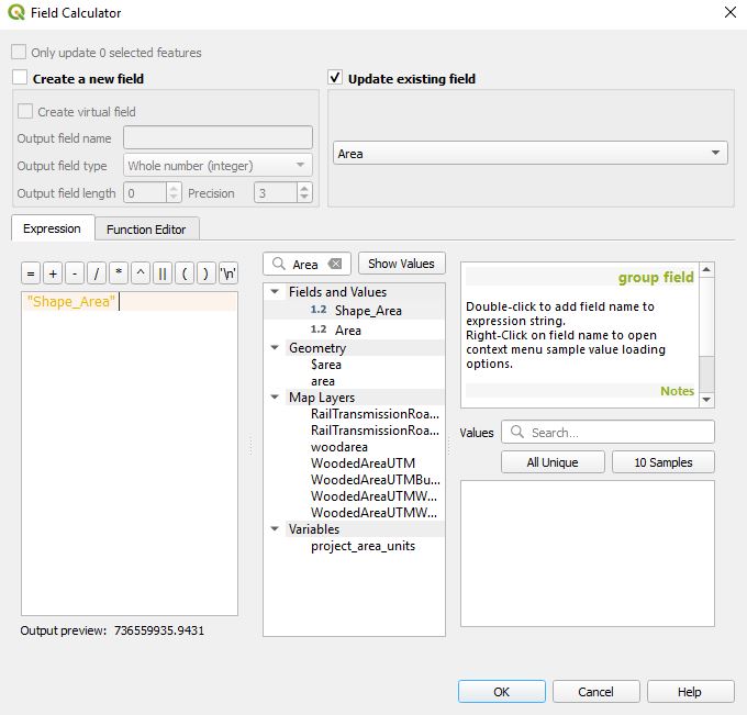
   3. Now open the 'Field Calculator' and select 'Update existing field' and select the field you created.
   4. In the search bar below, type in "area" and select the option named "$area"
   5. press 'OK' and all shapes will have an updated area field in meters squared. Sort the new field to find the largest in terms of area.
4. Once the largest suitable area has been identified, create a new vector polygon to represent this area. This can be done with the same process that was used to create the Ward 21 polygon from the Wards layer.

Representation of the Resulting Layer:

The resulting layer provides the largest suitable area for the specific region of interest with the consideration of all implied restrictions. By combining all the final layers together, you would get a map that shows the most suitable locations for wind turbines, along with the provincial restrictions set in place. This process can be used for any of the wards in the Ottawa region, and it could be used to select different areas with different restrictions, all depending on the data present.

Final output map

References

• Energy Ottawa. (2010). "Green Power". Accessed online: http://www.energyottawa.com/forms/index.cfm?dsp=template&act=view3&template_id=46&lang=e
• Ministry of the Environment, Conservation and Parks. "Location/site considerations checklist for renewable energy projects" Accessed online: https://www.ontario.ca/page/locationsite-considerations-checklist-renewable-energy-projects
• Natural Resources Canada. (2009). “Hydroelectric Generation”. The Atlas of Canada. Accessed online:http://atlas.nrcan.gc.ca/auth/english/maps/freshwater/consumption/hydroelectric/1