Difference between revisions of "Image Classification Tutorial using Orfeo Toolbox"
m |
|||
| (136 intermediate revisions by 3 users not shown) | |||
| Line 14: | Line 14: | ||
===Data Access=== |
===Data Access=== |
||
The first step in this tutorial is to download the free imagery |
The first step in this tutorial is to find and download the free imagery you will be using. Multiple sources are available online but for the purpose of this tutorial, the imagery was retrieved from Geobase, an up-to-date database of quality geospatial data for all of Canada. Landsat orthoimages acquired in August 2001 with less than 10% cloud, covering the nation's capital were downloaded and will be utilized for the supervised classification. Table 1 consists of a snapshot of the metadata for the images used in this tutorial. |
||
{| border="1" cellpadding="5" cellspacing="0" align="center" |
{| border="1" cellpadding="5" cellspacing="0" align="center" |
||
|+'''Table 1. Snapshot of the metadata for the five Landsat images obtained from Geobase''' |
|||
|+'''Landsat 7 Orthoimage''' |
|||
|- |
|- |
||
! style="background:#efefef;" | Dataset |
! style="background:#efefef;" | Dataset |
||
| Line 51: | Line 50: | ||
<br> |
<br> |
||
The orthorectified GeoTIFFs obtained from Geobase were already in an appropriate format and projection for our application therefore no image pre-processing was needed. For the purpose of this tutorial, the following bands were downloaded: |
|||
* Band 1 (Blue-green), 30 metres |
|||
* Band 2 (Green), 30 metres |
|||
* Band 3 (Red), 30 metres |
|||
* Band 4 (Near Infrared), 30 metres |
|||
* Band 8 (Panchromatic), 15 metres |
|||
===Orfeo Toolbox=== |
|||
====Installation==== |
|||
[[image:fig1.png|thumb|center|Orfeo Toolbox GUI]] |
|||
OTB is a multiplatform package which can be downloaded at http://www.orfeo-toolbox.org. The ready-to-install Windows binary package was downloaded, however, development version of OTB are also available for download, as well as a Quantum GIS plugin. Once OTB has been installed successfully, the software may be opened and the simple GUI is now displayed to the user. |
|||
<br> |
|||
====Insert Data==== |
|||
The GUI is simple and clean making it easy to navigate between tools. Once open, the next step involves inserting the Landsat bands previously downloaded from the Geobase website. |
|||
* Open the File menu and select Open Dataset |
|||
* Navigate to the folder where your Landsat bands are located and select one of the five TIFF files. Unfortunately, only one band may be inserted at a time, therefore this process will need to be repeated until all bands are inserted. The data type is automatically updated upon selecting your TIFF file. |
|||
Once all TIFF files have been opened, the GUI should display all five TIFFs in five separate Readers as seen in Figure 1. Within each reader there are two expandable folders, one RGB folder and one Grayscale folder. |
|||
::[[image:fig1.png|thumb|none|300px|Figure 1. Orfeo Toolbox GUI]] |
|||
<br> |
|||
====View Bands in RGB==== |
|||
Now that all the files are imported into OTB, you need to view them in RGB, but first all the imported files should be renamed in order to facilitate any further processing. Table 2 indicates the new fill name for all the bands. |
|||
*To change the band filename, expand the Greyscale folder of every inserted TIFF and right click on the file (i.e. 016028_0100_010825_l7_01_utm18 (band 1)) and select '''rename'''. |
|||
{| border="1" cellpadding="5" cellspacing="0" align="center" |
|||
|+'''Table 2. New filename given to the five bands downloaded from Geobase''' |
|||
|- |
|||
! style="background:#efefef;" | Band Orginal Name |
|||
! style="background:#efefef;" | New Name |
|||
! style="background:#efefef;" | Spectral Range |
|||
|- |
|||
| 016028_0100_010825_l7_01_utm18 |
|||
| Band 1 |
|||
| .45 to .515 (Blue) |
|||
|- |
|||
| 016028_0100_010825_l7_02_utm18 |
|||
| Band 2 |
|||
| .525 to .605 (Green) |
|||
|- |
|||
| 016028_0100_010825_l7_03_utm18 |
|||
| Band 3 |
|||
| .63 to .690 (Red) |
|||
|- |
|||
| 016028_0100_010825_l7_04_utm18 |
|||
| Band 4 |
|||
| .75 to .90 (NIR) |
|||
|- |
|||
| 016028_0100_010825_l7_08_utm18 |
|||
| Band 8 |
|||
| .52 to .90 (Pan) |
|||
|- |
|||
|} |
|||
* Write the appropriate name in the '''new instance label''' box. Once all the TIFFs have been renamed, all the files may be concatenated in order to view them in RGB. |
|||
* Open the File menu and select '''Concatenate Images'''. |
|||
* Add all the bands to the new image by selecting them individually and clicking the plus symbol. Once complete, you may modify the label name of the new image. As seen in Figure 2, all bands should be included. |
|||
::[[image:concatenate.png|thumb|none|400px|Figure 2. Concatenate Menu]] |
|||
* Once the all the bands have been concatenated, a new folder named Ottawa is added to the main GUI which contains all the bands. |
|||
* To display the bands in RGB, right click on the RGB folder (i.e. OutputImage) and select Display in Viewer. |
|||
* Two windows should open; one will display the image while the other contains the image setup. In order to properly view the RGB image, make sure the RGB composition mode is selected in the image setup window and the appropriate RGB bands are inserted in the Red, Green, and Blue Channels. See Figure 3 for an example of the RGB setup. |
|||
::[[image:rgb.png|thumb|none|400px|Figure 3. RGB Composition Mode]] |
|||
* By selecting on the Histogram tab in the image setup window, you have the option to modify the scaling parameters of the image therefore visually modifying the image to enhance natural color viewing capabilities. Having both the viewer window and setup window side by side is suggested in order to facilitate processing. |
|||
* To navigate the image, click on your desired area in the Navigation View in the viewer window, doing so will refresh the full resolution view. |
|||
* At this stage, it is suggested to export your RGB file comprised of all 5 bands. To do so, right click on the RGB Ottawa folder and select Export Dataset. Navigate to an appropriate folder and give the RGB file a name with its appropriate extension (i.e. ottawa.tif). Change the data type to 8bit unsigned in order to limit the size of the file (Landsat provides a maximum of 8 bits of reflectance data). |
|||
<br> |
|||
====Create your Area of Interest==== |
|||
Before being able to process the supervised classification, you need to set the extent of the area of interest (AOI). |
|||
* On the main title bar, select File>'''Extract ROI from dataset'''. |
|||
* Select your newly created concatenated file. Cache the Image in order to increase processing time. |
|||
* In the Select the ROI dialog box, create a box covering your AOI by dragging the cursor over the image. When satisfied with your AOI extent, click OK. Figure 4 contains an exmaple of the ROI dialog box |
|||
::[[image:aoi.png|thumb|none|400px|Figure 4. Region of Interest Dialog Box]] |
|||
* Save your AOI image by exporting the dataset as was done in the previous step. |
|||
<br> |
|||
====Clustering==== |
|||
In order to have a better understanding of the extent of the land-cover present in the image, a clustering algorithm will be processed to group spatially and spectrally the pixels of the AOI. Although this tool is better utilized when using high resolution imagery such as Ikonos or Quickbird, Landsat provides a freely available alternative. |
|||
* On the main title bar, select the Filtering menu>'''Mean Shift Clustering''' and select your AOI layer. |
|||
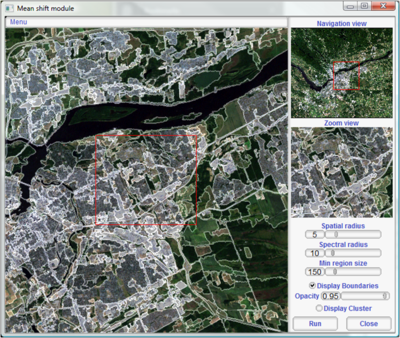
* In the mean shift module dialog box, several parameters may be adjusted in order to obtain the desired image. For this purpose of this tutorial and considering we are using a medium resolution image, you will only increase the Min region size to 150. By checking the Display Boundaries and Display Cluster, you can view the boundaries and cluster generated by the algorithm. The opacity option allows you to adjust the transparency in order to visualize the original image along with the boundaries as seen in Figure 5. Before closing the Mean Shift module, run the algorithm. The Mean Shift algorithm will create 2 images, a clustered and filtered image; both are added to your GUI. |
|||
::[[image:clustering.png|thumb|none|400px|Figure 5. Mean Shift Dialog Box]] |
|||
* Save the clustered image by following the export procedures demonstrated earlier. We will use the clustered image for the classification. |
|||
<br> |
|||
====Image Classification==== |
|||
To run a supervised classification, you will utilize the Support Vector Machines (SVM) algorithm in order to classify land-cover. The SVM approach seeks to locate optimal separating regions between classes by focusing on training polygons that are located on the edge of land-cover classes (Zhang and Ma, 2008). |
|||
* On the main title bar, select the Learning menu>'''SVM Classification''' and select your clustering layer. |
|||
* In the Supervised Classification dialog box, start by adding your first land-cover class by clicking on the '''Add''' function. By navigating on the image window, construct polygons over the corresponding land-cover. After drawing an individual polygon, you must click on '''End Polygon''' before moving on to the next one. |
|||
* You may rename your training class by clicking on the Name function and change the class polygon color all located under the '''Edit Classes''' menu. |
|||
For the purpose of this tutorial, the following five land-cover classes are created each with 4 to 8 training areas: water, forest, urban, agriculture and short vegetation |
|||
* You can take advantage of the 5 bands downloaded by using various RGB combinations to develop a greater understanding of the land covers in your study area. False colour composite (using bands 4, 3, and 2) and the panchromatic band may be employed in function of their advantages in depicting spectral information unavailable in natural color band combinations. |
|||
* After training polygons have been collected for the five classes as seen in Figure 6, you may return to your training areas if you need to delete any polygons using the '''Delete''' function or '''Erase Last Point''' tool to delete your last polygon vertex. You may also remove a class by simply selecting it and clicking on Remove. |
|||
::[[image:classification.png|thumb|none|400px|Figure 6. Supervised Classification Dialog Box]] |
|||
* If selected, the algorithm will create a random validation set in order to validate to classification result. |
|||
* After you are satisfied with your classes and training areas, click on Learn to start the classification. By clicking on Display, you can view the classification result in the viewer. The result will be added to the GUI and can now be saved. |
|||
* The final step in the classification involves the validation. By clicking on the Validation button, the algorithm will create a Confusion Matrix and Accuracy result based on your classified image and random validation set. |
|||
<br> |
<br> |
||
=== |
===Quantum GIS=== |
||
====Image Filter and Data Export==== |
|||
In this stage, you will apply a modal filter using a 5x5 window to the classification output to smooth out the spectral variability encountered by the classifier. Since OTB does not have a filter which successfully smoothes out the classification output generated by the SVM algorithm, the output was exported as a TIFF and imported in Quantum GIS. The following step involves processing raster layers within Quantum GIS with the Grass plugin. |
|||
====Installation==== |
|||
* Using the Grass Plugin, import the TIFF using '''r.in.gdal.qgis''' and add it as a layer to QGIS. |
|||
* Using '''r.colors.table''', assign a color table to the raster layer in order to visualize each land-cover class. |
|||
* After colors have been assigned to land-covers, use '''r.neighbors''' to apply a mode neighbourhood operation using a window size of 5 which replicates a mode filter often found in remote sensing software such as PCI Geomatica. Comparison between the original classification and filtered classification is displayed in Figure 7. |
|||
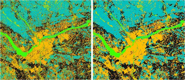
::[[image:Picture1.jpg|thumb|none|600px|Figure 7. Left is the unfiltered image and right is the result of the modal filter using a 5x5 window]] |
|||
* After the raster as been filtered, convert the raster to vector polygons using '''r.to.vect.area''' and add the resulting vector layer to Quantum GIS. This process may take several minutes depending on the amount of clusters and extent of your classification. |
|||
====View Bands in RGB==== |
|||
* In order to have to ability to share the vector layer on the internet with your various stakeholders, export the vector layer as KML. KML files enables you to view your vector dataset in Google Earth. To export the vector file to KML, use the '''v.out.ogr''' module. The resulting land-cover map may now be opened in Google Earth as seen in Figure 8. |
|||
::[[image:final_kml.jpg|thumb|none|400px|Figure 8. Land-cover classification viewed in Google Earth]] |
|||
:: '''''Note''': You may have to reproject your vector to the appropriate project (i.e. UTM) in order to properly view your KML file within Google Earth. Also, it is important to consider the symbology of your vector dataset before exporting to KML in order to facilitate visualization in Google Earth.'' |
|||
====Create your Area of Interest==== |
|||
====Clustering==== |
|||
* Depending on your vector output, Google Earth may not properly display large complex polygons, if so; you may have to cut large polygons in two or more smaller polygons in order for Google Earth to display the dataset. |
|||
====Image Classification==== |
|||
<br> |
|||
:: '''''Alternate procedure''': If needed, the land-cover vector file may be separated into multiple vector files each representing an individual land-cover. By exporting each individual land-cover separately to KML, the user has the ability to view individual land-covers by deactivating individual land-cover layers.''''' |
|||
===Quantum GIS=== |
|||
====Image Filter and Data Export==== |
|||
==Conclusion== |
==Conclusion== |
||
Congratulations, you have completed a supervised image classification using open source software and freely available Landsat imagery. Although many remote sensing applications rely on |
Congratulations, you have completed a supervised image classification using open source software and freely available Landsat imagery. Although many remote sensing applications rely on proprietary software because they have been tested and proven, this tutorial demonstrates that OTB software, although perhaps not yet mainstream, provides an open source alternative in an industry where large sums of money is spent purchasing proprietary software. While the SVM algorithm provided visually pleasing results, the incorporation of other supervised classifiers in OTB is needed to suit the different needs of various projects. By incorporating QGIS, the user has greater capabilities to manage and export data. QGIS proved to be an effective open source software to export data to KML and filtering imagery. Although OTB contains an option to export to KML, QGIS offers the opportunity to convert to vector which enhances the viewing capabilities of geospatial datasets in Google Earth. Overall, OTB offers valuable tools for image classification. It is designed to process high resolution imagery, however high resolution is often expensive with restrictive licenses, therefore use of such data falls outside the scope of this exercise. |
||
==References== |
==References== |
||
| Line 126: | Line 208: | ||
* [http://www.carleton.ca/ Carleton University] Web site |
* [http://www.carleton.ca/ Carleton University] Web site |
||
* [http://en.wikipedia.org/wiki/Carleton_University Carleton University Wiki] |
* [http://en.wikipedia.org/wiki/Carleton_University Carleton University Wiki] |
||
[[Category:Tutorials]] |
|||
Latest revision as of 10:49, 5 March 2012
Contents
Disclaimer
The information contained in this wiki is part of a project deliverable for a 4000 level Geomatics course at Carleton University. Information pertaining to software tools and parameters may be different depending on your application and software version. Landsat imagery was used in this tutorial however other image sources may be used to conduct this tutorial. Geospatial processing time may vary depending on computer configuration and size of data used.
Introduction
A fundamental aspect of image interpretation and analysis is the classification of land features in order to produce land cover maps. Typically produced using satellite imagery, classification is the process of sorting image pixels of unknown identity into groups based on points of known identity (Davidson, 2010). The user attempts to classify various features and/or land cover classes of interest using visual interpretation to group homogeneous pixels to create a thematic map (Canada Centre for Remote Sensing, 2008). Classification procedures can be broken into two categories based on the method used. Unsupervised classification, which determines natural statistical groupings within multispectral data based on the separations between means, is often used when little is known about the study area. Spectral classes are determined using statistical information followed by the user matching the classes to the land covers. Several algorithms can be employed to perform an unsupervised classification to determine the natural pixel groupings in the image. Supervised classification which can be seen as the reverse of unsupervised classification, involves the selection of land cover groupings to be mapped in combination with the delineation of training pixels for each class, the user has greater control over the procedure and has input on every step of the classification process compared to the unsupervised classification method. Once the training areas are delineated, a classifier such as maximum likelihood is used to assign all unknown pixels to the class whose training data they resemble most. The purpose of this tutorial is to emulate the supervised classification procedure using Orfeo Toolbox (OTB) and export the classification results in order to create thematic maps.
Background
This tutorial is conducted using Orfeo Toolbox. Orfeo Toolbox is an open source remote sensing image processing software with a goal of facilitating the development of new algorithms and validation procedures. It is a multiplatform, free to use software with a C++ library containing a multitude of pre-processing and image analysis algorithms. The graphical user interface or GUI provides non programmers with the ability to visually comprehend and analyze the procedures as well as interact with the available parameters. By including several well known algorithms and tools for free, OTB encourages research by stressing the importance of understanding how algorithms work, as their slogan puts it, OTB is not a black box (Orfeo Toolbox, 2010). OTB offers functionalities for remote sensing image processing such as but not limited to image filtering, feature extraction, change detection and classification.
Objective
In this tutorial you will learn how to apply your existing remote sensing skills to generate land-cover data using a supervised classification procedure in order to display the results in Google Earth using a combination of OTB and Quantum GIS (QGIS) with the Grass plugin. The final outcome is a KML file containing the land-cover polygons extracted from the supervised classification. Free and open source software and freely available Landsat imagery will be used to demonstrate an image classification application without using proprietary software.
Method
Data Access
The first step in this tutorial is to find and download the free imagery you will be using. Multiple sources are available online but for the purpose of this tutorial, the imagery was retrieved from Geobase, an up-to-date database of quality geospatial data for all of Canada. Landsat orthoimages acquired in August 2001 with less than 10% cloud, covering the nation's capital were downloaded and will be utilized for the supervised classification. Table 1 consists of a snapshot of the metadata for the images used in this tutorial.
| Dataset | Data Type |
|---|---|
| Product ID | 016026_0100_010825_L7Media_id |
| Projection | UTM_zone - 18 |
| Datum | NAD83 (CSRS) |
| Number of Pixels | 7602 |
| Raw Image Number | LE7016026000123750 Path - 016 |
| Acquisition Date | 2001/08/25 |
| Horizontal Positional Accuracy | 13 metres |
| Elevation Model Accuracy | 51 metres |
The orthorectified GeoTIFFs obtained from Geobase were already in an appropriate format and projection for our application therefore no image pre-processing was needed. For the purpose of this tutorial, the following bands were downloaded:
- Band 1 (Blue-green), 30 metres
- Band 2 (Green), 30 metres
- Band 3 (Red), 30 metres
- Band 4 (Near Infrared), 30 metres
- Band 8 (Panchromatic), 15 metres
Orfeo Toolbox
Installation
OTB is a multiplatform package which can be downloaded at http://www.orfeo-toolbox.org. The ready-to-install Windows binary package was downloaded, however, development version of OTB are also available for download, as well as a Quantum GIS plugin. Once OTB has been installed successfully, the software may be opened and the simple GUI is now displayed to the user.
Insert Data
The GUI is simple and clean making it easy to navigate between tools. Once open, the next step involves inserting the Landsat bands previously downloaded from the Geobase website.
- Open the File menu and select Open Dataset
- Navigate to the folder where your Landsat bands are located and select one of the five TIFF files. Unfortunately, only one band may be inserted at a time, therefore this process will need to be repeated until all bands are inserted. The data type is automatically updated upon selecting your TIFF file.
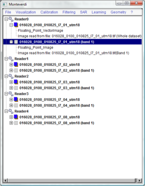
Once all TIFF files have been opened, the GUI should display all five TIFFs in five separate Readers as seen in Figure 1. Within each reader there are two expandable folders, one RGB folder and one Grayscale folder.
View Bands in RGB
Now that all the files are imported into OTB, you need to view them in RGB, but first all the imported files should be renamed in order to facilitate any further processing. Table 2 indicates the new fill name for all the bands.
- To change the band filename, expand the Greyscale folder of every inserted TIFF and right click on the file (i.e. 016028_0100_010825_l7_01_utm18 (band 1)) and select rename.
| Band Orginal Name | New Name | Spectral Range |
|---|---|---|
| 016028_0100_010825_l7_01_utm18 | Band 1 | .45 to .515 (Blue) |
| 016028_0100_010825_l7_02_utm18 | Band 2 | .525 to .605 (Green) |
| 016028_0100_010825_l7_03_utm18 | Band 3 | .63 to .690 (Red) |
| 016028_0100_010825_l7_04_utm18 | Band 4 | .75 to .90 (NIR) |
| 016028_0100_010825_l7_08_utm18 | Band 8 | .52 to .90 (Pan) |
- Write the appropriate name in the new instance label box. Once all the TIFFs have been renamed, all the files may be concatenated in order to view them in RGB.
- Open the File menu and select Concatenate Images.
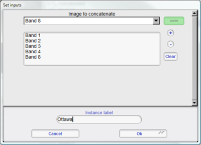
- Add all the bands to the new image by selecting them individually and clicking the plus symbol. Once complete, you may modify the label name of the new image. As seen in Figure 2, all bands should be included.
- Once the all the bands have been concatenated, a new folder named Ottawa is added to the main GUI which contains all the bands.
- To display the bands in RGB, right click on the RGB folder (i.e. OutputImage) and select Display in Viewer.
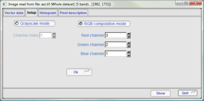
- Two windows should open; one will display the image while the other contains the image setup. In order to properly view the RGB image, make sure the RGB composition mode is selected in the image setup window and the appropriate RGB bands are inserted in the Red, Green, and Blue Channels. See Figure 3 for an example of the RGB setup.
- By selecting on the Histogram tab in the image setup window, you have the option to modify the scaling parameters of the image therefore visually modifying the image to enhance natural color viewing capabilities. Having both the viewer window and setup window side by side is suggested in order to facilitate processing.
- To navigate the image, click on your desired area in the Navigation View in the viewer window, doing so will refresh the full resolution view.
- At this stage, it is suggested to export your RGB file comprised of all 5 bands. To do so, right click on the RGB Ottawa folder and select Export Dataset. Navigate to an appropriate folder and give the RGB file a name with its appropriate extension (i.e. ottawa.tif). Change the data type to 8bit unsigned in order to limit the size of the file (Landsat provides a maximum of 8 bits of reflectance data).
Create your Area of Interest
Before being able to process the supervised classification, you need to set the extent of the area of interest (AOI).
- On the main title bar, select File>Extract ROI from dataset.
- Select your newly created concatenated file. Cache the Image in order to increase processing time.
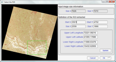
- In the Select the ROI dialog box, create a box covering your AOI by dragging the cursor over the image. When satisfied with your AOI extent, click OK. Figure 4 contains an exmaple of the ROI dialog box
- Save your AOI image by exporting the dataset as was done in the previous step.
Clustering
In order to have a better understanding of the extent of the land-cover present in the image, a clustering algorithm will be processed to group spatially and spectrally the pixels of the AOI. Although this tool is better utilized when using high resolution imagery such as Ikonos or Quickbird, Landsat provides a freely available alternative.
- On the main title bar, select the Filtering menu>Mean Shift Clustering and select your AOI layer.
- In the mean shift module dialog box, several parameters may be adjusted in order to obtain the desired image. For this purpose of this tutorial and considering we are using a medium resolution image, you will only increase the Min region size to 150. By checking the Display Boundaries and Display Cluster, you can view the boundaries and cluster generated by the algorithm. The opacity option allows you to adjust the transparency in order to visualize the original image along with the boundaries as seen in Figure 5. Before closing the Mean Shift module, run the algorithm. The Mean Shift algorithm will create 2 images, a clustered and filtered image; both are added to your GUI.
- Save the clustered image by following the export procedures demonstrated earlier. We will use the clustered image for the classification.
Image Classification
To run a supervised classification, you will utilize the Support Vector Machines (SVM) algorithm in order to classify land-cover. The SVM approach seeks to locate optimal separating regions between classes by focusing on training polygons that are located on the edge of land-cover classes (Zhang and Ma, 2008).
- On the main title bar, select the Learning menu>SVM Classification and select your clustering layer.
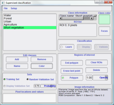
- In the Supervised Classification dialog box, start by adding your first land-cover class by clicking on the Add function. By navigating on the image window, construct polygons over the corresponding land-cover. After drawing an individual polygon, you must click on End Polygon before moving on to the next one.
- You may rename your training class by clicking on the Name function and change the class polygon color all located under the Edit Classes menu.
For the purpose of this tutorial, the following five land-cover classes are created each with 4 to 8 training areas: water, forest, urban, agriculture and short vegetation
- You can take advantage of the 5 bands downloaded by using various RGB combinations to develop a greater understanding of the land covers in your study area. False colour composite (using bands 4, 3, and 2) and the panchromatic band may be employed in function of their advantages in depicting spectral information unavailable in natural color band combinations.
- After training polygons have been collected for the five classes as seen in Figure 6, you may return to your training areas if you need to delete any polygons using the Delete function or Erase Last Point tool to delete your last polygon vertex. You may also remove a class by simply selecting it and clicking on Remove.
- If selected, the algorithm will create a random validation set in order to validate to classification result.
- After you are satisfied with your classes and training areas, click on Learn to start the classification. By clicking on Display, you can view the classification result in the viewer. The result will be added to the GUI and can now be saved.
- The final step in the classification involves the validation. By clicking on the Validation button, the algorithm will create a Confusion Matrix and Accuracy result based on your classified image and random validation set.
Quantum GIS
Image Filter and Data Export
In this stage, you will apply a modal filter using a 5x5 window to the classification output to smooth out the spectral variability encountered by the classifier. Since OTB does not have a filter which successfully smoothes out the classification output generated by the SVM algorithm, the output was exported as a TIFF and imported in Quantum GIS. The following step involves processing raster layers within Quantum GIS with the Grass plugin.
- Using the Grass Plugin, import the TIFF using r.in.gdal.qgis and add it as a layer to QGIS.
- Using r.colors.table, assign a color table to the raster layer in order to visualize each land-cover class.
- After colors have been assigned to land-covers, use r.neighbors to apply a mode neighbourhood operation using a window size of 5 which replicates a mode filter often found in remote sensing software such as PCI Geomatica. Comparison between the original classification and filtered classification is displayed in Figure 7.
- After the raster as been filtered, convert the raster to vector polygons using r.to.vect.area and add the resulting vector layer to Quantum GIS. This process may take several minutes depending on the amount of clusters and extent of your classification.
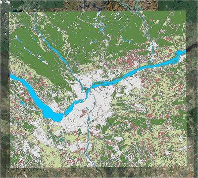
- In order to have to ability to share the vector layer on the internet with your various stakeholders, export the vector layer as KML. KML files enables you to view your vector dataset in Google Earth. To export the vector file to KML, use the v.out.ogr module. The resulting land-cover map may now be opened in Google Earth as seen in Figure 8.
- Note: You may have to reproject your vector to the appropriate project (i.e. UTM) in order to properly view your KML file within Google Earth. Also, it is important to consider the symbology of your vector dataset before exporting to KML in order to facilitate visualization in Google Earth.
- Depending on your vector output, Google Earth may not properly display large complex polygons, if so; you may have to cut large polygons in two or more smaller polygons in order for Google Earth to display the dataset.
- Alternate procedure: If needed, the land-cover vector file may be separated into multiple vector files each representing an individual land-cover. By exporting each individual land-cover separately to KML, the user has the ability to view individual land-covers by deactivating individual land-cover layers.
Conclusion
Congratulations, you have completed a supervised image classification using open source software and freely available Landsat imagery. Although many remote sensing applications rely on proprietary software because they have been tested and proven, this tutorial demonstrates that OTB software, although perhaps not yet mainstream, provides an open source alternative in an industry where large sums of money is spent purchasing proprietary software. While the SVM algorithm provided visually pleasing results, the incorporation of other supervised classifiers in OTB is needed to suit the different needs of various projects. By incorporating QGIS, the user has greater capabilities to manage and export data. QGIS proved to be an effective open source software to export data to KML and filtering imagery. Although OTB contains an option to export to KML, QGIS offers the opportunity to convert to vector which enhances the viewing capabilities of geospatial datasets in Google Earth. Overall, OTB offers valuable tools for image classification. It is designed to process high resolution imagery, however high resolution is often expensive with restrictive licenses, therefore use of such data falls outside the scope of this exercise.
References
Davidson, A. (2010). A Davidson's slides on Image Classification. GEOM 4003: Remote Sensing of the Environment.
Orfeo Toolbox. (2010). Orfeo Toolbox is not a black box.. Retrieved November 19, 2010 from http://www.orfeo-toolbox.org/otb/
Tutorial: Fundamentals of Remote Sensing Image interpretations & analysis - Image Classification. (2008). Canada Centre for Remote Sensing. Retreived November 19, 2010 from http://www.ccrs.nrcan.gc.ca/resource/tutor/fundam/chapter4/07_e.php
Zhang, R. & Ma, J. (2008). An improved SVM method P-SVM for classification of remotely sensed data. International Journal of Remote Sensing 29, 6029-6036
Related Links
- Orfeo Toolbox Web site
- Orfeo Toolbox Wiki
- Quantum GIS Web site
- Quantum GIS Wiki
- Grass GIS Web site
- Grass GIS Wiki
- Geobase Web site
- Geobase Wiki
- Google Earth Web site
- Google Earth Wiki
