Creating Maps in Jupyter Notebook using GeoPandas

Introduction

Aim

This tutorial will demonstrate how Jupyter Notebook can be used to manage and display spatial data in conjunction with Anaconda, GeoPandas, and QGIS. Using Jupyter Notebook in this procedure will enable you to develop your skills in scripting and automatic mapping while also learning more about open-source GIS software that is available. More specifically, this will involve using dynamic coordinate data to keep up-to-date maps and organize them in scripted notebooks. This workflow is accessible to users with less computational power, and data will be easier to store and manage. In the second part of this tutorial, we will show you how to display the data as a complete map (utilizing basic cartographic elements) in QGIS. This tutorial is designed for GIS users with some experience using graphic user interfaces, who are looking to get into using Python to streamline their workflow. The instructions and figures included in this tutorial were developed on the Windows operating system. If you are using a different operating system, your process may be slightly different.

About Jupyter

Jupyter Notebook was created by Project Jupyter, which is a collective which aims to develop open-source software in various programming languages. Jupyter Notebook specifically enables users to easily create and share code, as well as visualise data, among other uses. It is free to download and use (Jupyter, n.d.). While it runs in web browsers, it also runs locally on the user’s machine, which makes it easy to save version controls locally. Another advantage of Jupyter is that you can type code into kernels, and run those kernels individually. This will be demonstrated in the tutorial, but as a quick explanation -- the benefits to this include being able to test code easily and quickly visualize a certain data table, or in our case, create a map quickly without having to run all of the code at once. The main strength of Jupyter that we will be highlighting in this tutorial is its utility in visualising data that is updated frequently. The most pertinent example we have of that today are the daily updates in cases of COVID-19, which have been very effectively communicated through the use of maps.

About GeoPandas and CartoPy

GeoPandas is an open source library in Jupyter that builds off of pandas in Python. It is designed for users to more easily perform geospatial operations, by taking advantage of data frames in pandas, and creating spatial data frames. GeoPandas uses fiona for accessing files, Shapely objects for geometric manipulation and Matplotlib for plotting (geoPandas, n.d.). CartoPy is an open source package in Python that is designed for geospatial data processing. It takes advantage of shapely and NumPy libraries, and also uses matplotlib for plotting. It easily transforms points, lines and polygons based on geospatial projections, which helps virtualize and visualize data.

About QGIS

QGIS is a free and open-source comprehensive desktop GIS software with a wide variety of features that facilitate the display, analysis, and publishing of spatial data (QGIS, n.d.). In the context of this tutorial, QGIS enables us to expand on the work done in Jupyter by harnessing QGIS’ cartographic tools to produce a finished map with basic cartographic elements that can be saved and reused on updated iterations of the data.

Note on Software Versions

This tutorial uses the latest versions of software available at the time of writing (December 2020). The QGIS version used here is 3.16 Hannover, Python 3.9, and geoPandas 0.8.0. If you find updated versions of software when you try this tutorial, please note that there may be some differences in what you see in our screenshots and instructions, and what you see on your software.

Part 1: Getting Started

Software

This tutorial will be for Windows machines. The following steps will assume that the user is on a Windows platform, and therefore if you are using any other machine, the steps may be slightly different.

Install Anaconda

Install Anaconda here. You may also choose to simply install miniconda which will run everything necessary for the purpose of this tutorial, and most Jupyter notebook commands. You can install miniconda here in silent mode (recommended). Silent mode will automatically accept default settings and allow for quicker installation.

Install Jupyter Notebook

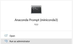
Next, you will need to install Jupyter Notebook.This can be done easiest through the Command Line in Windows. To open this up, you can search for “Anaconda Prompt” in the Windows Start Menu, and right-click “Run as Administrator” on the Anaconda Command Prompt application.

Figure 1.1. How to open Anaconda Prompt.

Install Jupyter Notebook in your users file directory by “Changing Directory” using cd to where you want to install it and using the following command:

conda install -c conda-forge jupyterlab

Install GeoPandas

Install the GeoPandas library using the same Anaconda Prompt application as used before. You should “Change Directory” using the cd prompt to where you would like geopandas to be installed. For the purpose of this tutorial, I will be installing it into a working folder, however I recommend installing both Jupyter Notebook and GeoPandas somewhere permanent in your file directory that will be easy to navigate to in the future, for example your users folder. Once in your desired file directory, install the latest version of GeoPandas using:

conda install geopandas

Figure 1.2. How to install GeoPandas.

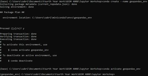
Next, we will be creating a new environment for geopandas. This is optional, but also recommended as good practise, as you may have dependency conflicts from previous installs of other software on your machine. This way, we can have a fresh start. To do this, enter the following command:

conda create --name [name of environment]

(Note: -n and --name is the same syntax)

Once created, you can activate this environment using:

conda activate [name of environment]

Figure 1.3. Setting up the GeoPandas environment.

Next, configure the environment to work with packages and install GeoPandas within them. Use the following commands, accepting the defaults with y.

conda config --env --add channels conda-forge

conda config --env --set channel_priority strict

conda install python=3 geopandas

Install Matplotlib and CartoPy

These packages will allow us to plot. Install them by running:

conda install -c conda-forge matplotlib

conda install -c conda-forge cartopy

conda install -c conda-forge descartes

Data

Download the following data and save the .csv files into your working directory:

John Hopkins COVID-19 Dataset:

Data Table

Part 2: Jupyter Notebook

Step 1: Introduction to Jupyter

Run Jupyter Notebook locally on your machine by searching for “Jupyter Notebook” in the Windows Start Menu. This will open up a terminal window that looks like Figure 2.1 below:

Figure 2.1. Opening up Jupyter.

It should also open up a new browser window automatically or you can use the URL provided above and copy & paste it into your browser.

Another way to open Jupyter Notebook is to use the following command in your working file directory:

jupyter-lab

Remember, that if you are ever running something in the command line and you want to stop running the process, ctrl + c will stop the process without having to restart your terminal.

Once opened, navigate to your working folder and Select “New” → Python 3 Notebook. This will open up a new tab where you can rename your project at the top and save.

Figure 2.2. Opening a new Notebook.

If you navigate back to the other tab, you will see something like the following (Figure 2.3):

Figure 2.3. Overview of working folder.

This shows a list of what is in your working folder. Here, we can see that the newly created notebook has been saved properly. If you navigate to the “Running” tab, you will see (Figure 2.4):

Figure 2.4. Overview of the Running tab.

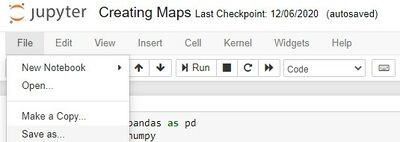
We should have one notebook running. This tab is useful to visualize what terminals and processes are running, and manage them accordingly. In the newly created notebook, we can see the top ribbon has many options (Figure 2.1). Here is a brief overview of some options you may find useful:

• Can change the title (“Creating Maps”)
• “File” has many useful options
• Typical new, save as, open, make a copy.
• The most useful feature is “Save and Checkpoint” where you can take advantage of Jupyter’s simple version controlling and then “Revert to Checkpoint”
• “Close and Halt” will close the notebook and halt it from running in the terminal (Note: if you open up the terminal again at any time while making changes to your notebook, you will see the changes being made locally on your machine)
• “Edit” and “Cell” helps move cells around, you can play around with these options or manually click and drag cells
• “Kernel” is important when running processes
• You can “Interrupt” the process (i.e if it is taking too long, or if you have noticed an error)
• You can “Restart and “Clear” it to get rid of any errors or outputs that may have come up

Step 2: Configuring the Data

In order to make our data usable and ready to be plotted, we need to first read it and slightly manipulate it. Copy this text into the first cell, replacing the red text in figure 2.5 with your [working directory/name of csv.csv].

import pandas as pd

import numpy as np

import matplotlib.pyplot as plt

from matplotlib import patheffects

from cartopy import crs as ccrs

import geopandas

import os

covid = pd.read_csv ([working directory/name of csv.csv])

world = geopandas.read_file(geopandas.datasets.get_path('naturalearth_lowres'))

Figure 2.5 Importing packages into Jupyter.

Here, we are importing all of the necessary packages, as well as assigning a variable name to our csv. We are also importing a world dataset from GeoPandas which we will be using to spatially merge to our csv, in order to map it.

You can run this cell, as well as the next two in order to see that the data has imported properly.

Figure 2.6 Individual cells to run in Jupyter.

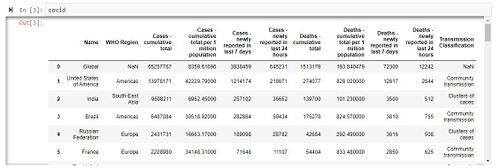
If you run these one at a time, you should see outputs like Figure 2.7:

Figure 2.7 Output of the covid cell.

Now that we have the two tables, we need to merge them by first, turning the Johns Hopkins dataset into a dataframe, and then renaming our country “Name” column to “name” using the following:

dfc = pd.DataFrame(covid)

df3 = dfc.rename({'Name': 'name'}, axis=1)

Figure 2.8 Syntax for turning the dataset into a dataframe and renaming columns.

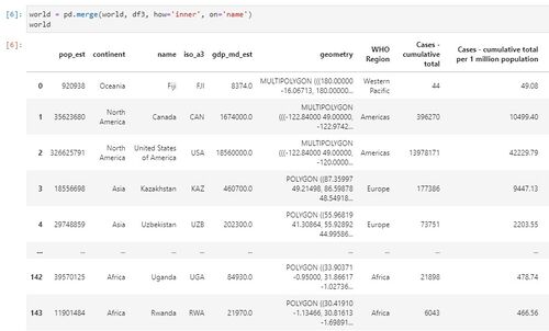
Next, we will spatially merge these datasets using the following:

world = pd.merge(world, df3, how='inner', on='name')

If you run this, you will see that they have been merged as shown below in Figure 2.9:

Figure 2.9 Output of the merge.

The first argument here is our “left” dataset, which is the geodataframe. The second is the “right” dataframe. ‘Inner’ refers to the retention of indices from both data frames, and we specified the ‘name’ column here.

Step 3: Displaying the Data

To display a map, simply enter:

covidworld = world.plot()

This will indicate any missing values, as well as will produce a basic map. However, to symbolize according to the Hopkins data, the following is required (Figure 2.10):

covidworld = world.plot(column='Cases - cumulative total per 1 million population',\

legend=True, legend_kwds={'shrink': 0.5}, figsize=(20, 15),\

missing_kwds={"color": "purple","edgecolor": "grey","hatch": "///","label": "Missing values"})

Figure 2.10 Configuring how the data is displayed.

This will symbolize by the cases per 1 million column, will display an appropriate legend, and resize the map, as well as shrink the legend proportionately and symbolize missing data values.

Conclusion

This tutorial explored how Jupyter Notebook and QGIS can be used together to facilitate the display of frequently updated spatial data. Below you can see the finished map showing the total cumulative cases of COVID-19 per 1 million population, using the streamlined workflow we developed in this tutorial.

For additional resources, check out these websites:

• GeoPandas Mapping Tools
• Interactive Maps in Jupyter Notebook
• Plotting with CartoPy and GeoPandas

References

GeoPandas. (n.d.). GeoPandas 0.8.0. Retrieved from https://geopandas.org/index.html

Jupyter. (n.d.). Jupyter. Retrieved from https://jupyter.org/

QGIS. (n.d.). Applications. Retrieved from https://www.qgis.org/en/site/about/features.html#qgis-desktop