Difference between revisions of "Using QGIS to conduct watershed analysis and 3D modeling"
Omargaweesh (talk | contribs) |
Omargaweesh (talk | contribs) |
||
| Line 378: | Line 378: | ||
| − | [6] " |
+ | [6] "Tool Upslope Area / SAGA-GIS Tool Library Documentation (v7.1.1)", Saga-gis.org, 2020. [Online]. Available: http://www.saga-gis.org/saga_tool_doc/7.1.1/ta_hydrology_4.html. |
Revision as of 00:00, 25 December 2020
Contents
Introduction and purpose
The purpose behind this tutorial is to show how QGIS can be used to conduct watershed analysis and how to create a 3D model of the Catchment area of the watershed using DEMs (Digital Elevation Model). This tutorial is meant to educate the user on how to conduct the analysis while introducing the theory behind it in a very simple manner in order for the user to understand the theory and apply the tutorial at the same time.
Acquiring DEMs
There are many websites that allow users to acquire DEMs, as a Carleton student, your best website you can use is the Geospatial Data Library of Carleton University linked HERE. Carleton University grants its student access to all sorts of geospatial data through its library and third parties like Scholars GeoPortal. For the purpose of this tutorial, I have found a DEM of rivers in Malaysia and will provide you with a link to the DEM if you would like to follow along. The link to the DEM can be downloaded from HERE.
Plug-ins installation
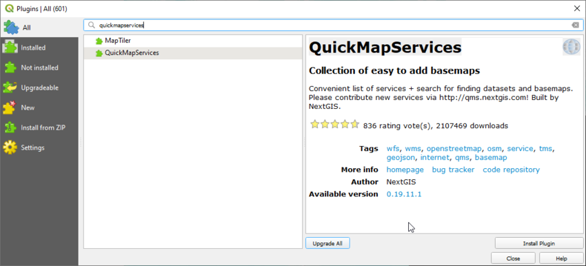
To help us reference the position of our DEM when we add it to our layers tab, the plug-in QuickMapServices will help us find easy and quick basemaps.
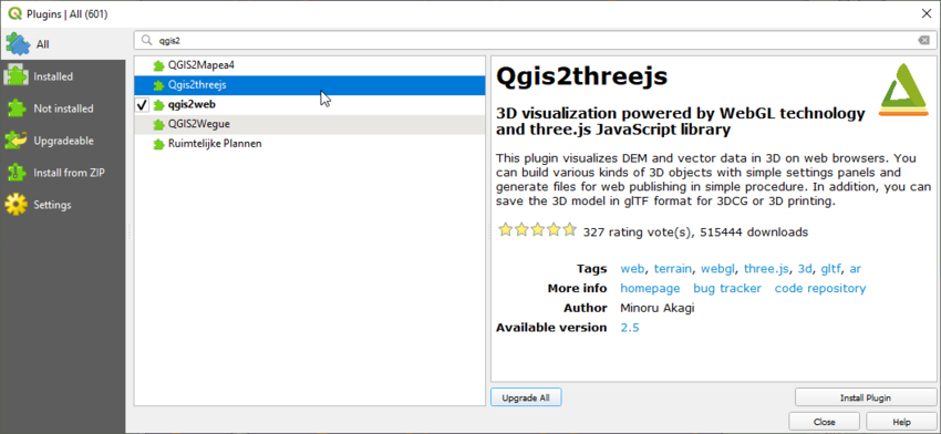
And to help us with 3D modeling, we will install the plug-in Qgis2threejs, which will use the elevation values in our DEM to create a 3D model of our catchment area.
Adding DEM and projecting
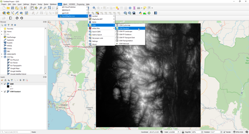
Once we add our DEM.tif file to our Layers, we use QuickMapServices to add a basemap. From our drop down menus, Web > QuickMapServices > OSM > OSM Standard. This will display Open Street Map in the backgound of our DEM as shown below:
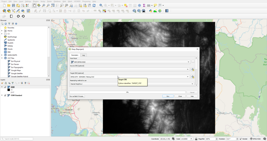
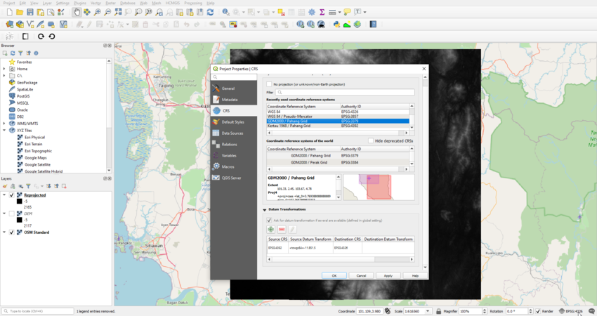
Next, we re-project our DEM to the appropriate projection, in our case -Malaysia- we can use GDM2000/Pahang Grid. Raster> Projections > Warp (Reproject) > Select GDM2000/Pahang Grid for target CRS. And from the bottom right hand corner, click on the projection icon, which will open the Project Properties, under CRS, chose GDM2000/Pahang Grid again.
After we are done with projections, the old DEM layer can be removed and we can rename the reporjected layer, for the sake of simplicity, it will be renamed Reprojected_DEM.
Now that we have our DEM ready, we can start the analysis!
Watershed Analysis
Step 1: Filling Sinks
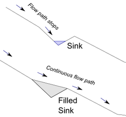
The very first step on our analysis is to what is called as Fill Sinks. The Fill Sinks tool by Wang & Liu produces a DEM free of depressions (AKA sinks) that would capture the flow of water, hence, conserving the waterflow in our data. The figure below is an example of a model with a "Sink" vs the same surface after filling the "Sink" and overland flow is continuous, which can be shown on Saga GIS tutorials website.[1]
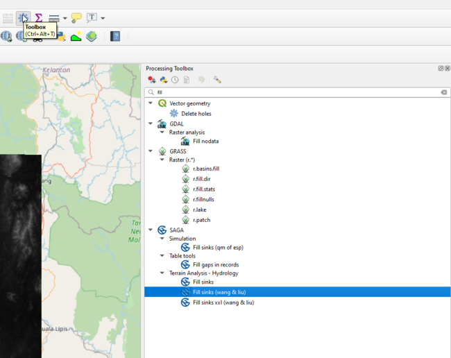
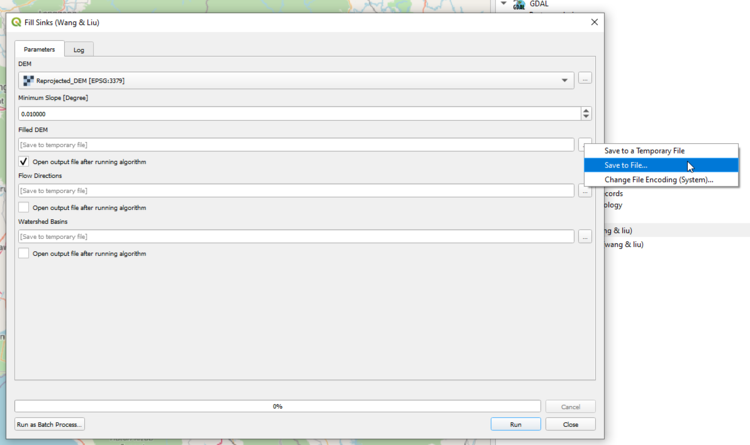
From Tools > SAGA > Fill sinks (wang & liu). Make sure to select the Reprojected_DEM and untick every option except (Open output file after running algorithm) and save to file using the 3 doted icon next to it. Hit RUN
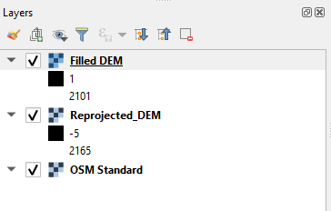
Notice the difference in our min and max values between the Filled DEM and our Reprojected_DEM:
Step 2: Strahler Order
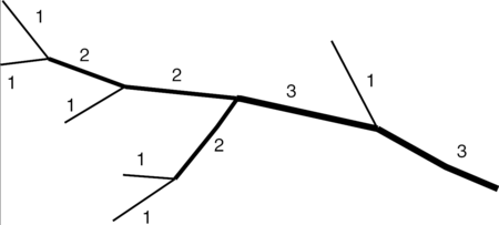
According to the system made by Strahler [2] [3], rivers of the first order are the outermost tributaries. If two streams of the same order meet, the resulting stream is given a number that is one higher. If two rivers of different stream orders meet, the resulting stream gets the higher of the two numbers. The following diagram showcases how Strahler Order works:
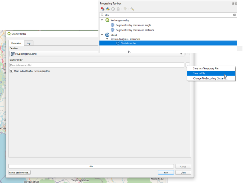
From Tools > SAGA > Strahler Order make sure to select the Filled DEM and tic (Open output file after running algorithm) and save to file using the 3 doted icon next to it. Hit RUN
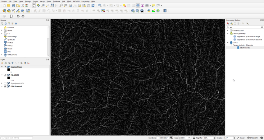
The resulting raster looks like this:
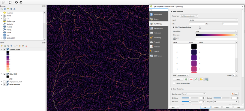
As we can see from the image above, Strahler Order identified 9 stream orders (1 to 9 under the raster layer) and it can be noted that some steams are brighter then others (Higher in Order). In order to make more sense of our 9 stream orders, we can change the Symbology of our raster. From the layer properties > Symbology. Change render type to Singleband pseudocolor and choose a color ramp that you like. Change Mode to Equal Interval and the number of classes to 9 as shown in the figure below:
Now we have a better view of our stream orders, where the darker ones are smaller in order and the lager ones go up from dark purple to yellow.
Depending on the analysis, we might not want to add the insignificant low streams in our analysis. Since Strahler Order assigns stream orders for each stream, we can use Raster Calculator to eliminate the the insignificant low streams.
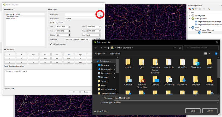
From the drop down menus, go to Raster > Raster Calculator, the following menu shows up:
From Raster Bands, select Strahler Order@1 and for the sake of our tutorial, we are interested in streams that are larger than or equal to 6. Make sure to save the result by clicking of the 3 doted icon highlighted in the image above.
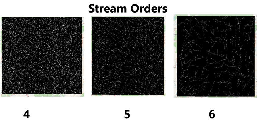
For the sake of demonstration, I have repeated this step for streams >= 4, >=5 and >=6 with the results shown below:
As we can see from the image above, a stream order of 6 included our main rivers and looked the best. We will use stream order of 6 in our analysis going forward and will be referred to as SO6 (OrderMoreThan6 in the screenshots).
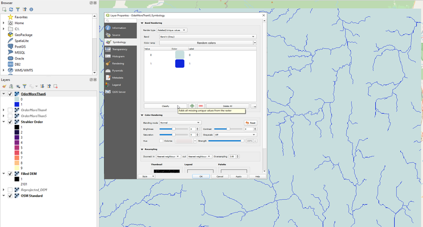
We can further improve the visibility SO6 by adjusting the Symbology: layer properties > Symbology. Change render type to Platted (Unique Values), then click on classify to show our unique values. Notice that running Raster Calculation resulted in 2 unique values of 0 (not river) and 1 (River) as it combined all of the SO6 streams into 1 river/stream.
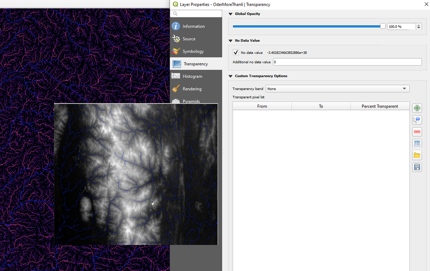
To make the most out of our SO6 symbology, we can make the Non-river pixels transparent by going to layer properties > Transparency > Additional no data value : 0 > Apply/Ok. That results in the non-river pixels being fully transparent and we can clearly see our SO6 highlighted in blue over our old DEM for reference as shown below:
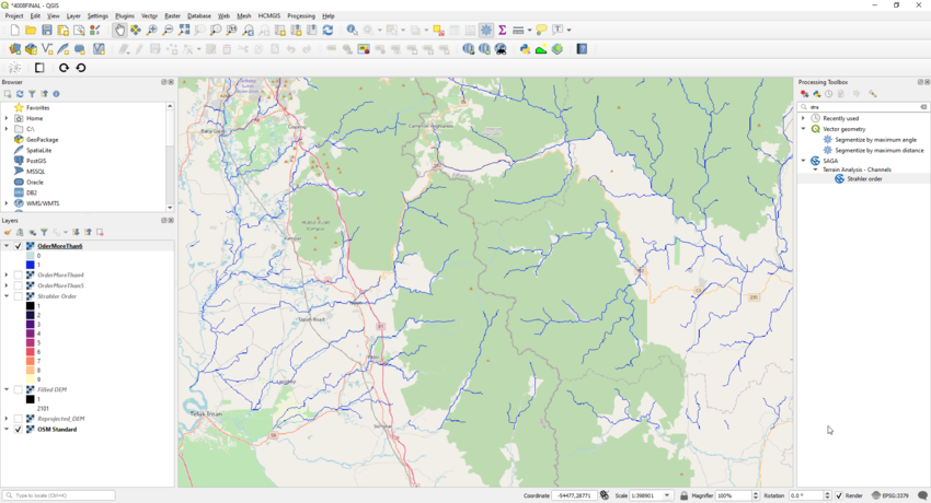
Here is an image of SO6 over the basemap:
Step 3: Channel network
After isolating SO6, we save our river network as a shapefile using the SAGA tool Channel network and Drainage basins. This tool can do more than that, as it can show the Strahler Order and even the direction of the water flow. For the sake of our tutorial, we are only focused on the river network channels.
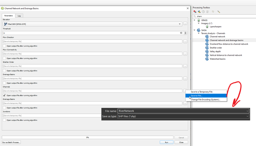
From the toolbox, search for Channel network and Drainage basins. Select Elevation to be our Filled DEM and set the threshold to 6 (The stream order), uncheck everything except Channels and save file as a Shapefile as shown below:
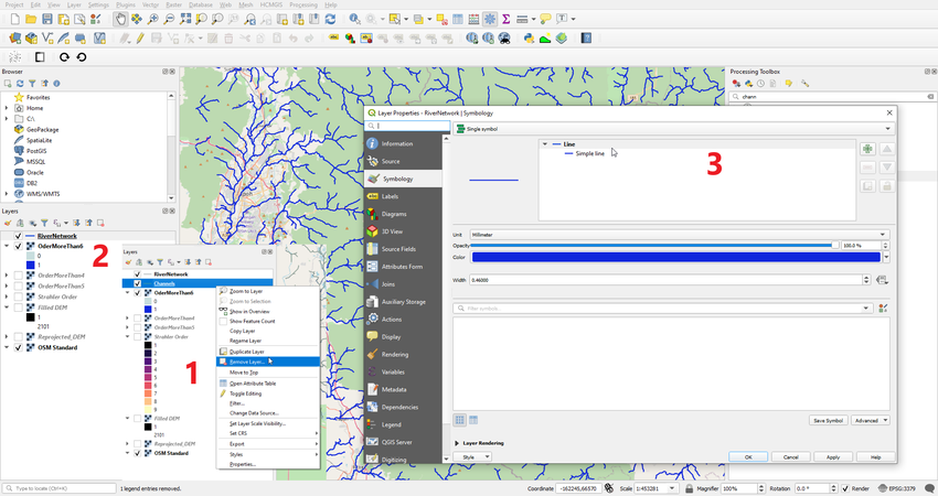
Feel free to delete the Channel layer produced by our tool. Go to your folder where you saved the shapefile and add that to the layers. I named the shapefile RiverNetwork and gave it a thicker blue line in symbology as shown below:
Step 4: Catchment areas / Drainage basins
After acquiring our shapefile RiverNetwork, we can now start to create catchment areas for points of interest. A drainage basin is any area where precipitation collects and drains off into one outlet, such as into a river, bay, or other body of water. The drainage basin includes all types of surface water like snowmelt, groundwater, rain runoff, and streams that run downslope towards that one outlet [5]. From the definition, we would need an outlet for us to conduct our analysis.
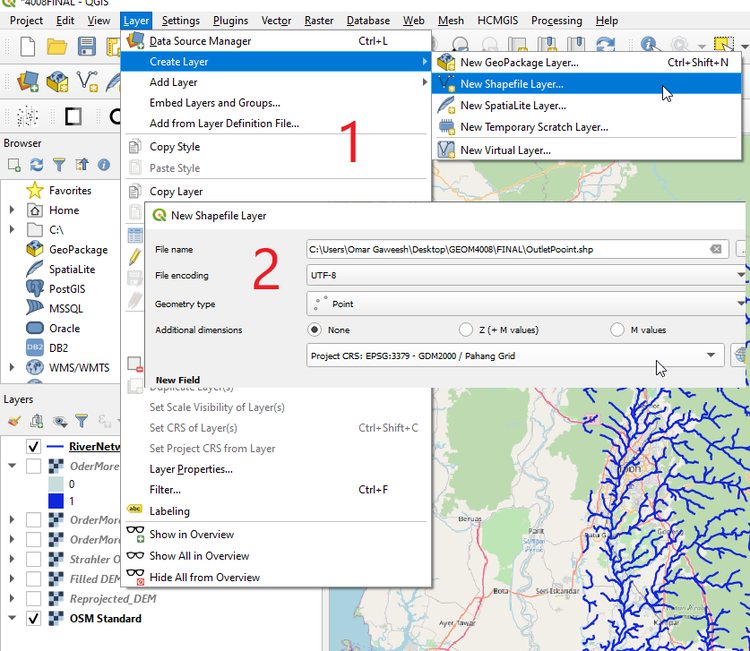
1- Create a point shapefile and make sure to select the proper projection as follows:
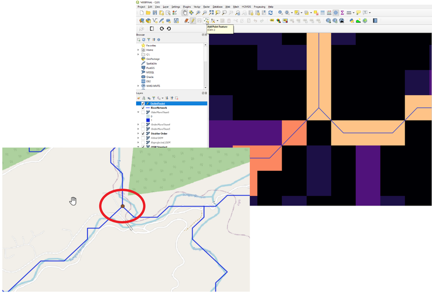
Make sure to show the old DEM pixels in order to pick the right stream that you are interested in, for the sake of our tutorial, I have selected a location in the middle of the river that had a high stream order (yellow), toggle editing and add you point where desired. (Notice that River network does not align perfectly everywhere, a higher quality DEM or the use of SAR imagery would result in higher quality results)
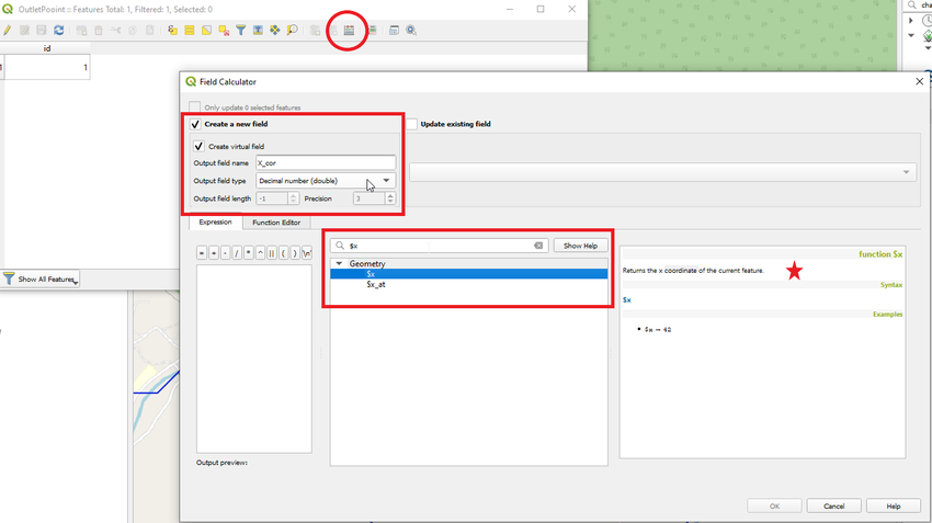
2- After saving our outlet point, go to the attributes table > field calculator. Make sure to add a new field, search for ($x) which returns the X coordinate of the feature. Change the output field type to Decimal number. Do the same for Y.
Result should be the X and Y coordinates as such:
3- Since we now have a river network and an outlet point, we can create our catchment area by using the SAGA tool Upslope Area.
Upslope Area allows users to specify target cells (in a lower elevation), for which the upslope contributing areas (higher elevation) shall be identified [6].
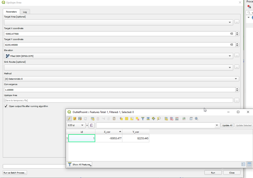
From the toolbox, search for Upslope Area, when the menu dialogue pops up, key in the target X and Y coordinates from the attribute table of our outlet point and choose the Filled DEM as our elevation as shown in the image below:
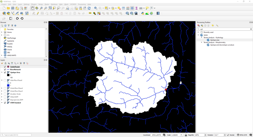
The following is the result of the Upslope analysis, you can see the outlet point in red, the RiverNetwork in blue and most importantly, the catchment area in white:
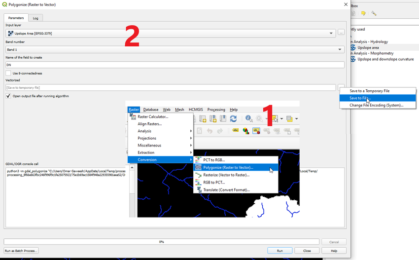
4- Since our result is still a raster, we can turn it into a polygon by going to the drop menu Raster > Conversion > Polygonize (Raster to Vector). Input layer should be the Upslope Area and the file should be saved as a shapefile.
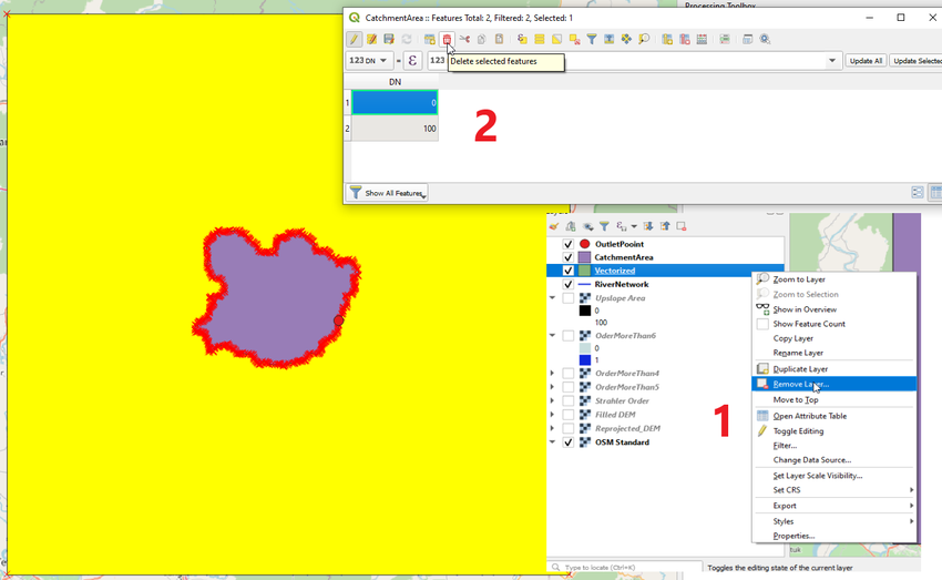
5- Add the shapefile that you just saved to your layers, them from attributes table, select the area outside your catchment area and hit delete (Note, you can delete the vectorized layer that is added by default).
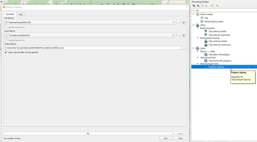
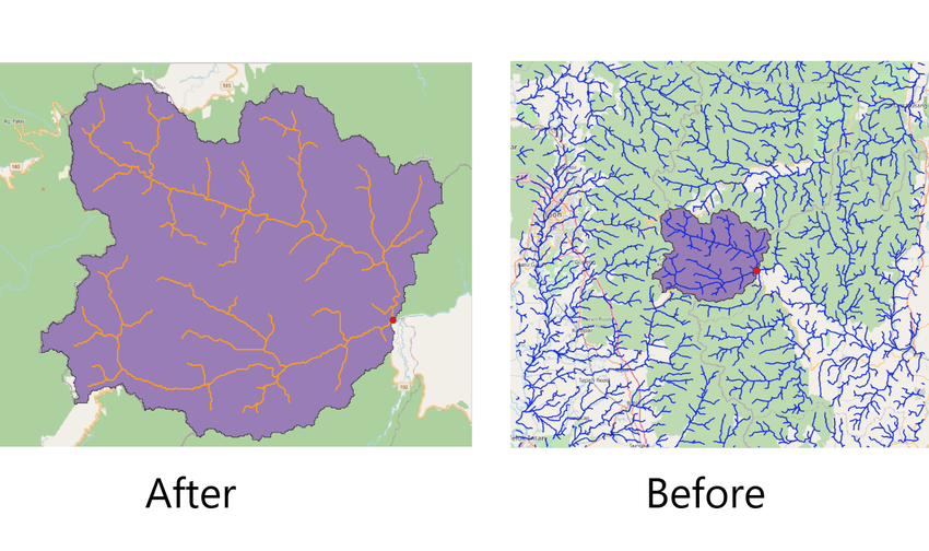
6- Clip the resulting shapefile with the RiverNetwork using the SAGA tool Polygon clipping as shown below:
Activate the layer RiverNetwork over the catchment area to see the final results.
With that done, we have successfully created a catchment area, where all those river streams pour into that outlet that we have selected! But what if we wanted to visualize that better, in 3D?
This is where 3D modeling comes into play!
3D Modeling of a DEM
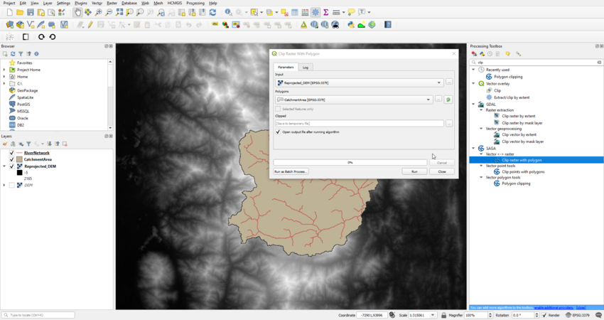
1- Using the Reprojected_DEM , the catchment area shapefile and the RiverNetwork we just created, we clip DEM raster to our catchment area shapefile using the SAGA tool Clip raster with polygon as shown in the image below:
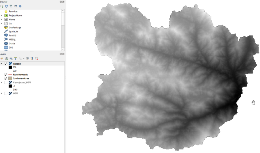
The clipped DEM looks like this:
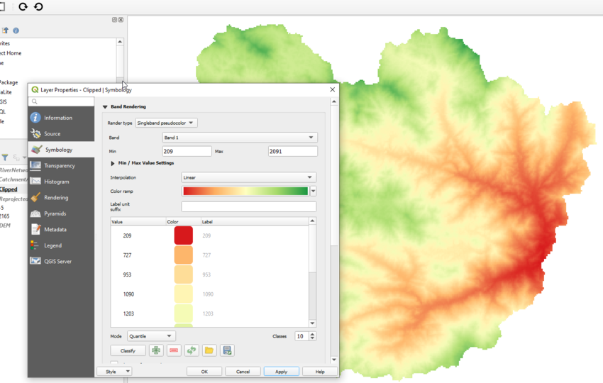
2- We can change the symbology of the DEM by introducing a color ramp to reflect the change in elevation. Set render type to Singleband pseudocolor and Mode to Quantile, chose an appropriate number of classes (example: 10), the result would be similar to the image below:
3- Time to 3D model!
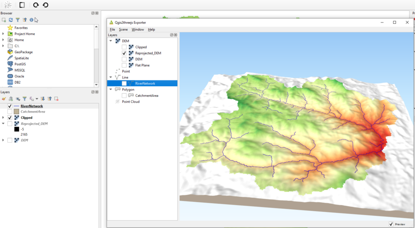
Using the plug-in tool Qgis2threejs that can be accessed through Web > Qgis2threejs > Qgis2threejs Exporter
Once activated, the Qgis2threejs Exporter window looks like this:
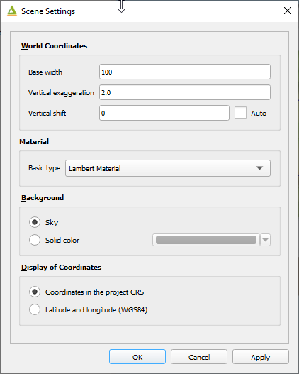
As we can see, Qgis2threejs created a 3D model of our DEM, but to further improve the 3D model, we can increase the Vertical Exaggeration from the default 1.0 to 2.0 or more as you see fit:
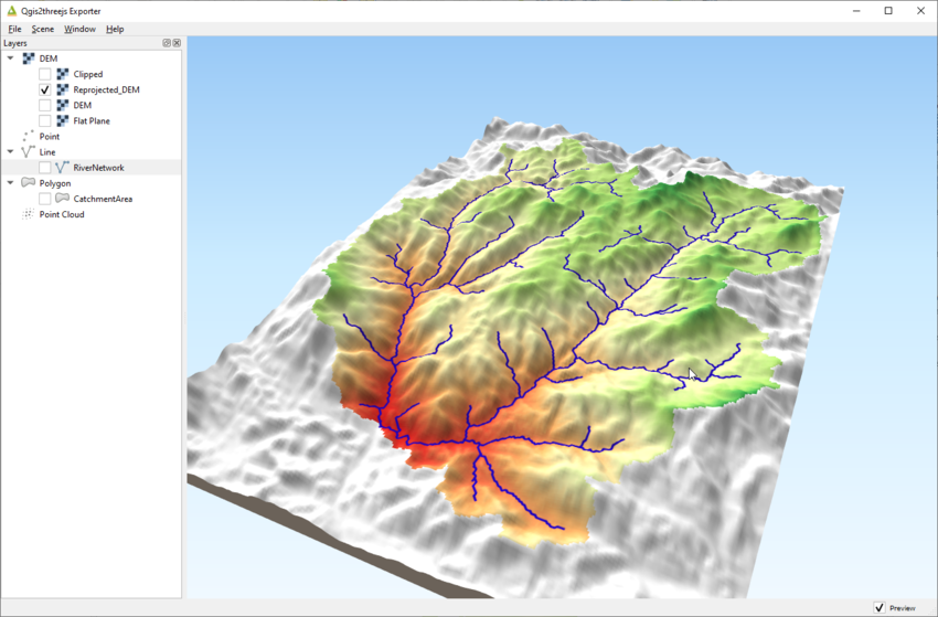
From our Layers, we can activate RiverNetwork to be able to view the final resulting 3D model, which looks like this:
Now we can easily understand how how watershed analysis works! streams with lower order in areas with higher elevation (Green) merge together forming higher order streams that flow down the slopes of higher elevations until we get to areas with lower elevations (Yellow to Red) where in our case, the streams on the right and the streams on the left merge together in our Outlet area (red).
References
[1] "Preprocessing and catchment deliniation", Saga GIS tutorials, 2020. [Online]. Available: https://sagatutorials.wordpress.com/preprocessing-and-catchment-deliniation/.
[2] Strahler, A.N. Quantitative analysis of watershed geomorphology. Transactions of the American Geophysical Union. 1957; 38(6), pp. 913-920.
[3] Strahler, A.N. "Quantitative geomorphology of drainage basins and channel networks." Chow, V.T., Editor. Handbook of Applied Hydrology. New York: McGraw-Hill; 1964; pp. 4-39, 4-76
[4] "Stream order", En.wikipedia.org, 2020. [Online]. Available: https://en.wikipedia.org/wiki/Stream_order.
[5] DeBarry, Paul A. (2004). Watersheds: Processes, Assessment and Management. John Wiley & Sons.
[6] "Tool Upslope Area / SAGA-GIS Tool Library Documentation (v7.1.1)", Saga-gis.org, 2020. [Online]. Available: http://www.saga-gis.org/saga_tool_doc/7.1.1/ta_hydrology_4.html.
