Difference between revisions of "Editing Vector Data in GRASS GIS"
SheaTimmins (talk | contribs) |
SheaTimmins (talk | contribs) |
||
| (41 intermediate revisions by the same user not shown) | |||
| Line 5: | Line 5: | ||
== Data == |
== Data == |
||
First we will need to download our data. You can download the Ottawa Traffic Collision data [https://open.ottawa.ca/datasets/ottawa::traffic-collision-by-location-2019/explore?location=45.250250%2C-75.806856%2C1.62 here.] After you proceed to the link, click the download button, and select "shapefile." Once you have downloaded the Traffic Collision data, click [https://open.ottawa.ca/datasets/ottawa::red-light-camera-violations-2019/explore?location=45.376580%2C-75.686783%2C2.96 here] to download the Red Light violations data. |
First we will need to download our data. You can download the Ottawa Traffic Collision data [https://open.ottawa.ca/datasets/ottawa::traffic-collision-by-location-2019/explore?location=45.250250%2C-75.806856%2C1.62 here.] After you proceed to the link, click the download button, and select "shapefile." Once you have downloaded the Traffic Collision data, click [https://open.ottawa.ca/datasets/ottawa::red-light-camera-violations-2019/explore?location=45.376580%2C-75.686783%2C2.96 here] to download the Red Light violations data. Finally, download the Road Centrelines data [https://open.ottawa.ca/datasets/ottawa::road-centrelines/explore?location=45.245509%2C-75.794650%2C1.87 here.] |
||
== Getting Started with Grass == |
== Getting Started with Grass == |
||
| Line 11: | Line 11: | ||
Start by launching the GRASS software. You should see three windows, one is a terminal, one is the Map Display, and one is the main interface that includes tabs along the bottom of the window such as "data" and "layer," which we will refer to as the Layer Manager for convenience. You need to add a new "database," which is essentially a folder that you will keep "locations" in. Within the "locations," you will store your mapsets. |
Start by launching the GRASS software. You should see three windows, one is a terminal, one is the Map Display, and one is the main interface that includes tabs along the bottom of the window such as "data" and "layer," which we will refer to as the Layer Manager for convenience. You need to add a new "database," which is essentially a folder that you will keep "locations" in. Within the "locations," you will store your mapsets. |
||
By default, you have a database named something similar to "C:\Users\YourUserName\Documents\grassdata." |
By default, you have a database named something similar to "C:\Users\YourUserName\Documents\grassdata." |
||
Once done, go back to the Layer's Interface window in GRASS, and select the "add new location" icon. |
Once done, go back to the Layer's Interface window in GRASS, and select the "add new location" icon. |
||
| Line 17: | Line 17: | ||
[[File:GRASS_newlocation1.png|400px]] |
[[File:GRASS_newlocation1.png|400px]] |
||
<br /> |
<br /> |
||
<br />Name your location " |
<br />Name your location "ottawa_road_safety" and click Next.<br /> |
||
<br /> |
<br /> |
||
[[File: |
[[File:ottawa_road_safety.png|400px]] |
||
<br /> |
|||
<br /> |
|||
Select "Select CRS from a list by EPSG or description" and press Next. |
|||
<br /> |
|||
<br /> |
|||
[[File:Selectingcoordinatesystem.png|400px]] |
|||
<br /> |
|||
<br /> |
|||
Chose NAD27(CGQ77)/UTM zone 19N. This is the ideal projection for the Ottawa area. Select Next, and then Finish. |
|||
<br /> |
|||
<br /> |
|||
[[File:UTMzone19.png|400px]] |
|||
<br /> |
|||
<br /> |
|||
You should now see a new location in your Layer Manager titled ottawa_road_safety. |
|||
<br /> |
|||
<br /> |
|||
[[File:allsetup.png|400px]] |
|||
<br /> |
|||
<br /> |
|||
Before we upload our data in GRASS, open your filefolder on your computer and make sure that the data you downloaded from open.ottawa.ca is in the correct folder location (i.e. C:\Users\YourUserName\Documents\grassdata\ottawa_road_safety\PERMANENT.) |
|||
<br /> |
|||
<br /> |
|||
Next, navigate back to the Layers Manager window in GRASS. Ensure that you are working in the correct location by right-clicking ottawa_roads_safety and selecting "switch mapsets." Next Select the icon shaped like a "V" to import vector data. |
|||
<br /> |
|||
<br /> |
|||
[[File:importV.png|300px]] |
|||
<br /> |
|||
<br /> |
|||
Select browse, and navigate to where you stored your downloaded data. Select the "Traffic_Collision_by_Location_2019.shp" file and select "Import." |
|||
<br /> |
|||
<br /> |
|||
[[File:importingshape1.png|400px]] |
|||
<br /> |
|||
<br /> |
|||
Select "Import and reproject" when prompted. |
|||
<br /> |
|||
<br /> |
|||
[[File:reproject1.png|400px]] |
|||
<br /> |
|||
<br /> |
|||
You should now see a display similar to the one below on your Map Display window. |
|||
<br /> |
|||
<br /> |
|||
[[File:mapdisplay1.png|600px]] |
|||
<br /> |
|||
<br /> |
|||
Repeat these same steps to import the Red Light Violations data; select the icon shaped like a "V." This time, after you select browse, and navigate to where you stored your downloaded data, select the "Red_Light_Camera_Violations_2019.shp" file and select "Import." Next, repeat this for the Road Centrelines data. At the end you should have two layers in your Layers tab. |
|||
<br /> |
|||
<br /> |
|||
[[File:layerstab1.png|600px]] |
|||
<br /> |
|||
<br /> |
|||
== Editing the Map Display == |
|||
First, make sure the layers are in the correct order. Roads_Centrelines.shp should be the bottom layer. If this is not the case, simply click and drag that layer to the beneath the other two. We are then going to edit our Map Display so that it displays the intersections and areas in Ottawa with a significant number of red light traffic violations and traffic violations in one year. |
|||
===Displaying Layers Based on Attribute Data=== |
|||
The first thing we will edit in our Map display is the Red_Light_Camera_Violations_2019.shp data. We are going to display only the intersections that have 500 or more traffic violations in the year of 2019. |
|||
Right-click on Red_Light_Camera_Violations_2019.shp and select "Properties." |
|||
<br /> |
|||
<br /> |
|||
[[File:redlight1.png|600px]] |
|||
<br /> |
|||
<br /> |
|||
Select the "Selection" tab. Then, underneath where it says (where=sql_query), select the blue and white rectangle/square icon. |
|||
<br /> |
|||
<br /> |
|||
[[File:sql_redlight.png|400px]] |
|||
<br /> |
|||
<br /> |
|||
Next, double click the TOTAL_VIOL column. Then select the >= sign, and type 500. Your final query should look like the one below. Press "Apply." |
|||
<br /> |
|||
<br /> |
|||
[[File:grassslqred.png|300px]] |
|||
<br /> |
|||
<br /> |
|||
Press "Apply" again. Then close the d.vect window. |
|||
<br /> |
|||
<br /> |
|||
[[File:montgomery.png|400px]] |
|||
<br /> |
|||
<br /> |
|||
If you uncheck the boxes for each layer except for the Red_Light_Camera_Violations_2019 layer, your map display should look like the one below. We have successfully displayed only the intersections with 500 or more violations in the year 2019. |
|||
<br /> |
|||
<br /> |
|||
[[File:stage1.png|700px]] |
|||
<br /> |
|||
<br /> |
|||
Now we will repeat these steps with the Traffic_Collision_by_Location_2019 layer. Right-click on this layer, and select "Properties." Next, select the "Selection" tab. Select the same square icon again underneath (where=sql_query). This time, double-click the Total_Coll column. Then select the >= button, and type 10. Select "Apply." Select "Apply" again then close the d.vect window. We have now set the Map Display to only display areas with 10 collisions or more in the year 2019. |
|||
<br /> |
|||
<br /> |
|||
[[File:collisions10.png|400px]] |
|||
<br /> |
|||
<br /> |
|||
===Editing Symbols=== |
|||
We will start by editing the Traffic_Collision_by_Location_2019 symbols on our Map Display. By default, they are the same color as the other layers, making the information very difficult to discern. We will start by changing the color of the symbol. Right-click on the Traffic_Collision_by_Location_2019 layer, and select “Properties.” Then select the “Colors” tab. It should look like the photo below. |
|||
<br /> |
|||
<br /> |
|||
[[File:colorz.png|400px]] |
|||
<br /> |
|||
<br /> |
|||
Click on the “Feature color.” Then select a new color, in the example below a bright green was selected. Click “OK” and then “Apply.” There is an example of what your Map Display should look like below. |
|||
<br /> |
|||
<br /> |
|||
[[File:colorzz.png|400px]] |
|||
<br /> |
|||
<br /> |
|||
[[File:mapz.png|400px]] |
|||
<br /> |
|||
<br /> |
|||
Now we will repeat these steps with the Red_Light_Camera_Violations_2019 layer. Right-click on this layer, and select “Properties.” Navigate to the “Colors” tab, and select a red color. Click “OK” and then “Apply.” Now your Map Display should look like the one below. |
|||
<br /> |
|||
<br /> |
|||
[[File:displayz.png|500px]] |
|||
<br /> |
|||
<br /> |
|||
Our data is concentrated in the downtown area of Ottawa, so we are going to zoom in this area to make our Display more readable. Select the magnifying glass at the top of your screen that has the plus sign. Then click the center of the most concentrated area of your map. The result on your map display should be similar to the one below. |
|||
<br /> |
|||
<br /> |
|||
[[File:yeehawz.png|500px]] |
|||
<br /> |
|||
<br /> |
|||
Next we are going to edit the symbol size and shape. Right-click on the Traffic_Collision_by_Location_2019 layer. Select “Properties,” then select the “Symbols” tab. Click on the “X” to change the shape of the symbol. Select the circle as the new symbol. Next change the symbol size to 6. Your “Symbols" tab should look like the photo below. |
|||
<br /> |
|||
<br /> |
|||
[[File:coloredit.png|400px]] |
|||
<br /> |
|||
<br /> |
|||
Before you press “Apply” and close this window, navigate back to the “Colors” tab and change the “Area fill color” to yellow. Then press apply. The Map Display should now look like the one below. |
|||
<br /> |
|||
<br /> |
|||
[[File:symbolstuff.png|500px]] |
|||
<br /> |
|||
<br /> |
|||
Now we will do the same thing for the Red_Light_Camera_Violations_2019 layer. Right-click on this layer, and select “Properties.” Then, go to the “Symbols” tab and change the symbol from “X” to a circle, and the size from 5 to 6. Before you press “Apply,” navigate to the “Colors” tab and select the color red for the “Area fill color.” You Map Display should now look like the one below. |
|||
<br /> |
|||
<br /> |
|||
[[File:peachtea.png|500px]] |
|||
<br /> |
|||
<br /> |
|||
==Conclusion== |
|||
In this tutorial, you have begun to explore ways of editing your map display in GRASS GIS. By the end of it, you should be more comfortable uploading data into GRASS, and editing symbols in vector layers. There is much more you can do in this program, and hopefully this tutorial gives you the confidence and the basics to continue to explore the features of GRASS. |
|||
Latest revision as of 14:23, 22 December 2022
Contents
Introduction
This tutorial will demonstrate how to do a vector analysis using GRASS GIS. By the end, you should be a little more comfortable using the program. Please note that for this tutorial we are using GRASS 8.2, older versions of GRASS may not reconcile with this tutorial. Our goal is to use the 2020 Red Light Camera Violations data from open.ottawa.ca to make a map that displays the safest areas in Ottawa to drive based on the number of traffic violations. If you do not already have GRASS installed on your computer, you can go to this Intro to GRASS workshop page with detailed instructions on how to download it.
Data
First we will need to download our data. You can download the Ottawa Traffic Collision data here. After you proceed to the link, click the download button, and select "shapefile." Once you have downloaded the Traffic Collision data, click here to download the Red Light violations data. Finally, download the Road Centrelines data here.
Getting Started with Grass
Start by launching the GRASS software. You should see three windows, one is a terminal, one is the Map Display, and one is the main interface that includes tabs along the bottom of the window such as "data" and "layer," which we will refer to as the Layer Manager for convenience. You need to add a new "database," which is essentially a folder that you will keep "locations" in. Within the "locations," you will store your mapsets.
By default, you have a database named something similar to "C:\Users\YourUserName\Documents\grassdata."
Once done, go back to the Layer's Interface window in GRASS, and select the "add new location" icon.
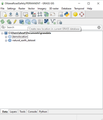
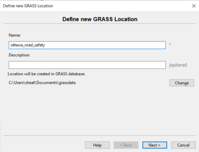
Name your location "ottawa_road_safety" and click Next.
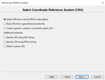
Select "Select CRS from a list by EPSG or description" and press Next.
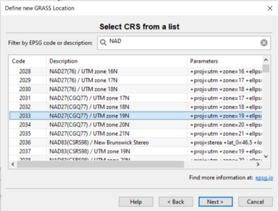
Chose NAD27(CGQ77)/UTM zone 19N. This is the ideal projection for the Ottawa area. Select Next, and then Finish.
You should now see a new location in your Layer Manager titled ottawa_road_safety.
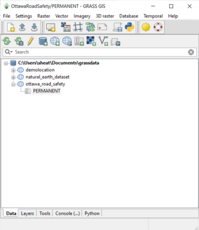
Before we upload our data in GRASS, open your filefolder on your computer and make sure that the data you downloaded from open.ottawa.ca is in the correct folder location (i.e. C:\Users\YourUserName\Documents\grassdata\ottawa_road_safety\PERMANENT.)
Next, navigate back to the Layers Manager window in GRASS. Ensure that you are working in the correct location by right-clicking ottawa_roads_safety and selecting "switch mapsets." Next Select the icon shaped like a "V" to import vector data.
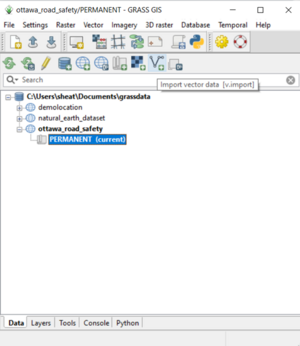
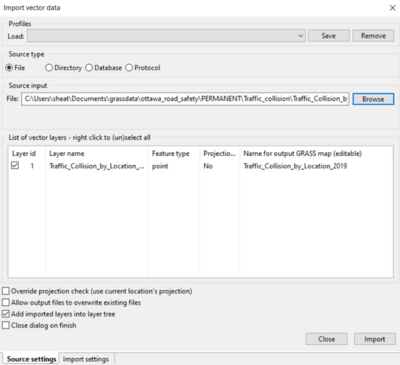
Select browse, and navigate to where you stored your downloaded data. Select the "Traffic_Collision_by_Location_2019.shp" file and select "Import."
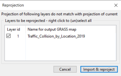
Select "Import and reproject" when prompted.
You should now see a display similar to the one below on your Map Display window.
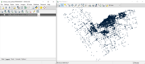
Repeat these same steps to import the Red Light Violations data; select the icon shaped like a "V." This time, after you select browse, and navigate to where you stored your downloaded data, select the "Red_Light_Camera_Violations_2019.shp" file and select "Import." Next, repeat this for the Road Centrelines data. At the end you should have two layers in your Layers tab.
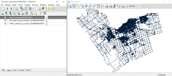
Editing the Map Display
First, make sure the layers are in the correct order. Roads_Centrelines.shp should be the bottom layer. If this is not the case, simply click and drag that layer to the beneath the other two. We are then going to edit our Map Display so that it displays the intersections and areas in Ottawa with a significant number of red light traffic violations and traffic violations in one year.
Displaying Layers Based on Attribute Data
The first thing we will edit in our Map display is the Red_Light_Camera_Violations_2019.shp data. We are going to display only the intersections that have 500 or more traffic violations in the year of 2019. Right-click on Red_Light_Camera_Violations_2019.shp and select "Properties."
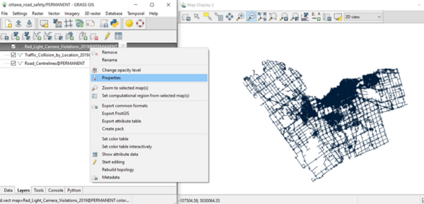
Select the "Selection" tab. Then, underneath where it says (where=sql_query), select the blue and white rectangle/square icon.
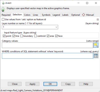
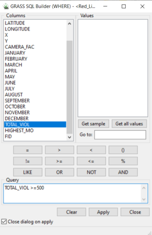
Next, double click the TOTAL_VIOL column. Then select the >= sign, and type 500. Your final query should look like the one below. Press "Apply."
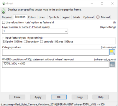
Press "Apply" again. Then close the d.vect window.
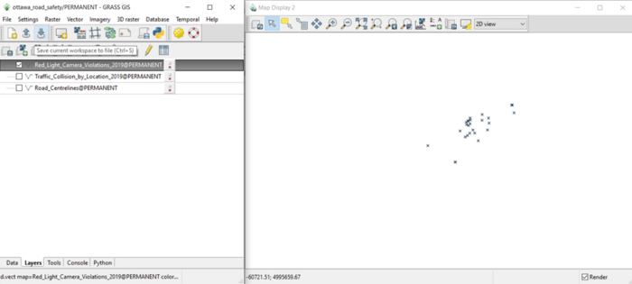
If you uncheck the boxes for each layer except for the Red_Light_Camera_Violations_2019 layer, your map display should look like the one below. We have successfully displayed only the intersections with 500 or more violations in the year 2019.
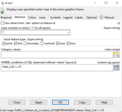
Now we will repeat these steps with the Traffic_Collision_by_Location_2019 layer. Right-click on this layer, and select "Properties." Next, select the "Selection" tab. Select the same square icon again underneath (where=sql_query). This time, double-click the Total_Coll column. Then select the >= button, and type 10. Select "Apply." Select "Apply" again then close the d.vect window. We have now set the Map Display to only display areas with 10 collisions or more in the year 2019.
Editing Symbols
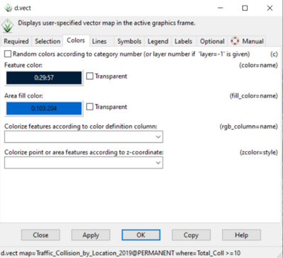
We will start by editing the Traffic_Collision_by_Location_2019 symbols on our Map Display. By default, they are the same color as the other layers, making the information very difficult to discern. We will start by changing the color of the symbol. Right-click on the Traffic_Collision_by_Location_2019 layer, and select “Properties.” Then select the “Colors” tab. It should look like the photo below.
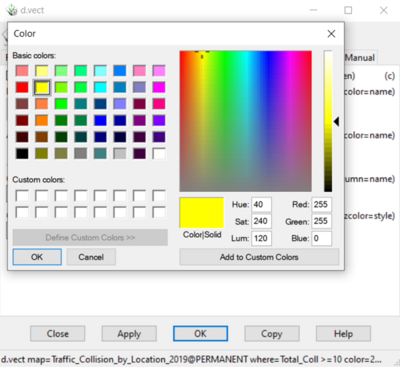
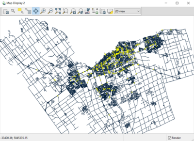
Click on the “Feature color.” Then select a new color, in the example below a bright green was selected. Click “OK” and then “Apply.” There is an example of what your Map Display should look like below.
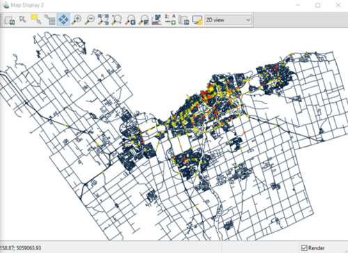
Now we will repeat these steps with the Red_Light_Camera_Violations_2019 layer. Right-click on this layer, and select “Properties.” Navigate to the “Colors” tab, and select a red color. Click “OK” and then “Apply.” Now your Map Display should look like the one below.
Our data is concentrated in the downtown area of Ottawa, so we are going to zoom in this area to make our Display more readable. Select the magnifying glass at the top of your screen that has the plus sign. Then click the center of the most concentrated area of your map. The result on your map display should be similar to the one below.
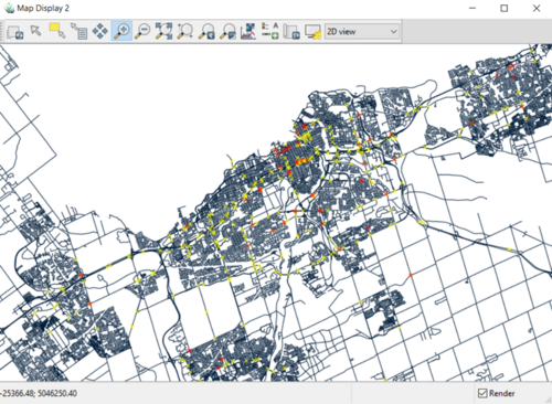
Next we are going to edit the symbol size and shape. Right-click on the Traffic_Collision_by_Location_2019 layer. Select “Properties,” then select the “Symbols” tab. Click on the “X” to change the shape of the symbol. Select the circle as the new symbol. Next change the symbol size to 6. Your “Symbols" tab should look like the photo below.
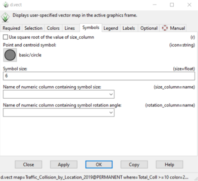
Before you press “Apply” and close this window, navigate back to the “Colors” tab and change the “Area fill color” to yellow. Then press apply. The Map Display should now look like the one below.
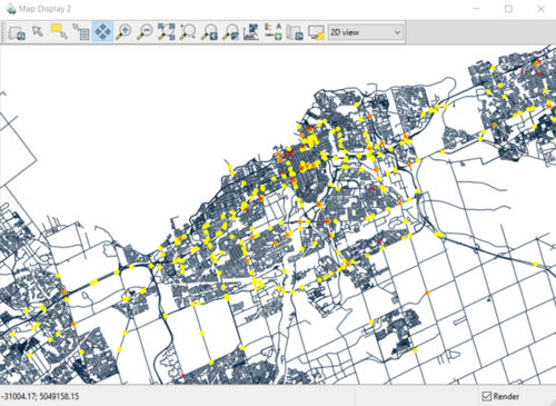
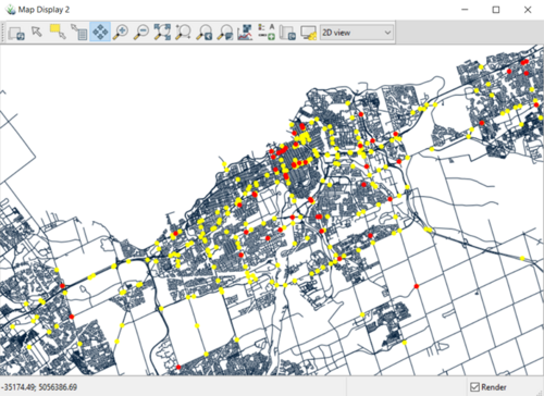
Now we will do the same thing for the Red_Light_Camera_Violations_2019 layer. Right-click on this layer, and select “Properties.” Then, go to the “Symbols” tab and change the symbol from “X” to a circle, and the size from 5 to 6. Before you press “Apply,” navigate to the “Colors” tab and select the color red for the “Area fill color.” You Map Display should now look like the one below.
Conclusion
In this tutorial, you have begun to explore ways of editing your map display in GRASS GIS. By the end of it, you should be more comfortable uploading data into GRASS, and editing symbols in vector layers. There is much more you can do in this program, and hopefully this tutorial gives you the confidence and the basics to continue to explore the features of GRASS.