Difference between revisions of "Utilizing Rstudio as an alternative GIS"
Razzroutly (talk | contribs) |
|||
| (23 intermediate revisions by 2 users not shown) | |||
| Line 17: | Line 17: | ||
=== QGIS === |
=== QGIS === |
||
We start by creating a fresh install of QGIS in order to download the functions that we will be exploring in this tutorial. QGIS can be installed from https://www.qgis.org/en/site/forusers/download.html, for the purposes of this tutorial we will be installing the 64-bit version. |
We start by creating a fresh install of QGIS in order to download the functions that we will be exploring in this tutorial. QGIS can be installed from https://www.qgis.org/en/site/forusers/download.html, for the purposes of this tutorial we will be installing the 64-bit version for Windows. For other operating systems, follow directions at the QGIS website. |
||
| ⚫ | |||
[[File:QGISinstall.PNG|600px|thumb|none| Figure 1: QGIS 64-bit installer.]] |
[[File:QGISinstall.PNG|600px|thumb|none| Figure 1: QGIS 64-bit installer.]] |
||
| Line 31: | Line 32: | ||
=== R and RStudio === |
=== R and RStudio === |
||
In order to utilize RStudio we first need to download '''R'''. This can be downloaded from https://cran.r-project.org/bin/windows/base/. For this installer we will be accepting all of the default paths and options. |
In order to utilize RStudio we first need to download '''R'''. This can be downloaded for Windows from https://cran.r-project.org/bin/windows/base/. For this installer we will be accepting all of the default paths and options. |
||
[[File:Rdownload 2023.png|600px|thumb|none| Figure 3: R 4.3.1 installer.]] |
[[File:Rdownload 2023.png|600px|thumb|none| Figure 3: R 4.3.1 installer.]] |
||
| Line 37: | Line 38: | ||
[[File:RStudioDownload 2023.png|600px|thumb|none| Figure 4: RStudio version 2023.09.0+463 installer.]] |
[[File:RStudioDownload 2023.png|600px|thumb|none| Figure 4: RStudio version 2023.09.0+463 installer.]] |
||
== RStudio |
== RStudio setup == |
||
Now that we have all of the software that we need we can proceed with setting up RQGIS within RStudio. In order to run QGIS functions within RStudio we will need to download and unpack some packages which allow for the manipulation of spatial data. After installing these packages within the workspace we will link our workspace with the root directory of QGIS in order to gain access to its host of functions and algorithms. |
Now that we have all of the software that we need we can proceed with setting up RQGIS within RStudio. In order to run QGIS functions within RStudio we will need to download and unpack some packages which allow for the manipulation of spatial data. After installing these packages within the workspace we will link our workspace with the root directory of QGIS in order to gain access to its host of functions and algorithms. |
||
=== Install Packages === |
=== Install Packages === |
||
Start by opening up RStudio and creating a new ‘’’R script’’’ file (file->new file->R script). Within this new script we will be downloading and installing some packages that allow us to manipulate raster and spatial data within RStudio. Start by adding this code to your script and running it. |
Start by opening up RStudio and creating a new ‘’’R script’’’ file (file->new file->R script). Within this new script we will be downloading and installing some packages that allow us to manipulate raster and spatial data within RStudio. Start by adding this code to your script and running it. |
||
#Install packages |
|||
install.packages("sp") |
install.packages("sp") |
||
install.packages(" |
install.packages("sf") |
||
install.packages(" |
install.packages("geodata") |
||
install.packages("qgisprocess") |
|||
install.packages("raster") |
install.packages("raster") |
||
install.packages("rgdal") |
install.packages("rgdal") |
||
#Attach packages to workspace |
|||
library("sp") |
library("sp") |
||
library(" |
library("sf") |
||
library(" |
library("geodata") |
||
library("qgisprocess") |
|||
library("raster") |
library("raster") |
||
library("rgdal") |
library("rgdal") |
||
*'''sp''': provides functions for plotting spatial data |
*'''sp''': provides functions for plotting spatial data |
||
*'''sf''': provides functions for using spatial features |
|||
| ⚫ | |||
*'''geodata''': provides open source spatial data used in the tutorial |
|||
*'''rgeos''': allows for the manipulation of vector data |
|||
| ⚫ | |||
*'''raster''': Provides the user to read, write and manipulate raster images within RStudio |
*'''raster''': Provides the user to read, write and manipulate raster images within RStudio |
||
*'''rgdal''': Provides the user to read, write and manipulate shapefiles within RStudio |
*'''rgdal''': Provides the user to read, write and manipulate shapefiles within RStudio |
||
=== Set workspace environment === |
|||
Now that we have installed all the necessary packages we have to link the directory of the QGIS applications to our current RStudio workspace. This is achieved by utilizing the set_env() function. |
|||
'''#Links QGIS paths to the current RStudio workspace''' |
|||
set_env() |
|||
Try adding this line to your script,after running this line the console should provide path names similar to this example. |
|||
| ⚫ | |||
Now you have full access to all of the geoprocessing functions found within your copy of QGIS Desktop. Within this workspace you will be able to call these functions to manipulate and display spatial data. |
|||
== Data Acquisition == |
== Data Acquisition == |
||
In this tutorial we will make use of datasets that are accessible within RStudio as a method of showcasing the use of various QGIS geoprocessing functions. In order to access these datasets you use the data() function which provides the user with a list of all available datasets preloaded within RStudio. Additionally, the getData() function allows the user to download geographic data for specific countries around the world. |
In this tutorial we will make use of datasets that are accessible within RStudio as a method of showcasing the use of various QGIS geoprocessing functions. In order to access these datasets you use the data() function which provides the user with a list of all available datasets preloaded within RStudio. Additionally, the getData() function allows the user to download geographic data for specific countries around the world. |
||
=== |
=== Setting Path === |
||
First we will create a folder within your main directory in order to store all of the outputs that we create within this tutorial. This folder will be placed in the first branch of your C: drive. If your computer's OS home directory is located on a different drive (such as a D: drive) you will have to modify the drive name within the code to match your situation. |
|||
First we will make sure the working directory is set to the C: drive of your computer. This can be done using the '''setwd("C:")''' command which will ensure all path based commands use the root C: directory as their base. You can also use this command to set the working directory for R as a different folder location, however this may cause problems if you have spaces in your file paths so use with caution. Additionally, we will make a variable called '''path''' which will point to the location that we want and input/output files to be stored. This path will then be used in subsequent commands by adding concatenating the string variable of the path with the name of the file, such as '''paste(path,"/output.txt", sep=""))'''. |
|||
'''#Create a working directory for this tutorial''' |
'''#Create a working directory for this tutorial''' |
||
setwd("C:") |
|||
path = "C:/Users/razzroutly/Documents/Classes/GEOM4008" |
|||
subDir <- "tutorial" |
|||
if (file.exists(subDir)){ |
|||
setwd(file.path(mainDir, subDir)) |
|||
} else { |
|||
dir.create(file.path(mainDir, subDir)) |
|||
setwd(file.path(mainDir, subDir)) |
|||
| ⚫ | |||
=== Importing Data === |
=== Importing Data === |
||
One of the advantages of using RStudio as an alternative GIS is its ability to load open source geospatial data with just one line of code. For this tutorial we will be using the '''geodata''' package to access digital elevation models using the elevation_30s() command which will provide a raster with 30 arc second (1km) from the Shuttle Radar Topography Mission, supplemented by GTOP30 data for high latitudes [https://rdrr.io/cran/geodata/man/elevation.html [1<nowiki>]</nowiki>]. |
|||
Next we will import the datasets that we will be using in this tutorial into our workspace and display them within the RStudio '''plot''' frame. We will be downloading a DEM of Canada as well as a preloaded DEM of Mt. Mongón which is located in Peru. The '''data()''' function allows the user to access a variety of datasets preloaded within Rstudio, whereas the '''getData()''' function downloads data from an online database. |
|||
'''#Digital elevation model (DEM) of the Mongón study area''' |
|||
We will import the dataset that used in this tutorial into our workspace and display it within the RStudio '''plot''' frame. We will be downloading a DEM of Canada from the '''geodata''' package. The '''getData()''' function downloads data from an online database. Due to the high resolution of the raster we will also use a function from the '''raster''' package that will aggregate the raster cells by a factor of 10 to make processing easier. |
|||
data(dem) |
|||
dem_mongon<-dem |
|||
| ⚫ | |||
'''#Digital elevation model (DEM) of Canada''' |
'''#Digital elevation model (DEM) of Canada''' |
||
canada_dem<-getData('alt', country='CAN', mask=TRUE) |
canada_dem<-getData('alt', country='CAN', mask=TRUE) |
||
plot(canada_dem, col=grey(0:100/100), main='DEM of Canada') |
plot(canada_dem, col=grey(0:100/100), main='DEM of Canada') |
||
canada_dem_agg <- aggregate(canada_dem, fact=10) |
|||
After running this code you will notice that the DEM's are displayed in the lower right '''plot''' window. The outputs should look like this: |
After running this code you will notice that the DEM's are displayed in the lower right '''plot''' window. The outputs should look like this: |
||
[[File:DEMCANADA1.png|500px |
[[File:DEMCANADA1.png|500px|thumb|none| Figure 6: DEM of Canada displayed within the plot window.]] |
||
| ⚫ | |||
. |
. |
||
== QGIS Functions == |
== QGIS Functions == |
||
In order to utilize QGIS functions within RStudio, we first have to learn how to find the functions we want to use with their respective syntax, as well as learn what parameters we will be working with for each function. In order to do this we will be making use of the ''' |
In order to utilize QGIS functions within RStudio, we first have to learn how to find the functions we want to use with their respective syntax, as well as learn what parameters we will be working with for each function. In order to do this we will be making use of the '''qgis_search_algorithms()''' and '''qgis_show_help()''' functions. The '''qgis_search_algorithms()''' function allows the user to enter a keyword for the function they are interested in using, and provides the user with a list of available functions that pertain to that keyword as well as which provider within QGIS they come from (SAGA, GDAL, GRASS, etc.), algorithims that are found in the base version of QGIS have the provider "native". After selecting the function that we are interested in using we can use the '''qgis_show_help()''' function to display a description of the use for the function as well as the input and output parameters that the function utilizes. As an example we will use the '''qgis_search_algorithms()''' function to search for a clipping function. |
||
'''#Searches for functions which contain the keyword 'clip'''' |
'''#Searches for functions which contain the keyword 'clip'''' |
||
qgis_search_algorithms(algorithm="clip") |
|||
find_algorithms(search_term = 'clip') |
|||
After running this line you will see a list of 11 clipping tools that have been displayed in the console. |
After running this line you will see a list of 11 clipping tools that have been displayed in the console. |
||
[[File: |
[[File:QGIS R algoSearch.png|500px|thumb|none| Figure 7: Clipping algorithms available for use within RStudio]] |
||
We will select the GDAL clipping function '''gdal:cliprasterbyextent''' and determine which parameters we will need to be able to make use of this function in RStudio. To do this we will use the '''qgis_get_argument_specs()''' function. In order to use this function we need to use the full name of the function which is '''gdal:cliprasterbyextent'''. |
|||
'''#Provides the user with information regarding the parameters of a function''' |
'''#Provides the user with information regarding the parameters of a function''' |
||
qgis_show_help("gdal:cliprasterbyextent") |
|||
get_usage(alg = "qgis:clip",intern=FALSE) |
|||
When running this line of code you will see a list of the functions parameters appear in the console. This provides you with information regarding the type of input required for each parameter and provides the user with a legend for parameters that are normally accessed through drop down boxes in QGIS. |
When running this line of code you will see a list of the functions parameters appear in the console. This provides you with information regarding the type of input required for each parameter and provides the user with a legend for parameters that are normally accessed through drop down boxes in QGIS. |
||
[[File: |
[[File:GDAL clip RStudio.png|500px|thumb|none| Figure 8: Description and parameters for GDAL cliprasterbyextent function in QGIS.]] |
||
| ⚫ | |||
| ⚫ | |||
| ⚫ | |||
| ⚫ | The first algorithm we will investigate is ''' |
||
| ⚫ | |||
| ⚫ | The first algorithm we will investigate is '''gdal:polygonize'''. This algorithm takes a raster image and converts its features into polygons. In order to use this function we will need to determine the parameters for: input, field, and output. The '''qgis_run_algorithm()''' function takes in the desired algorithm as well as that algorithms parameters, since the output of this function is very large we will be storing the output vector in the temporary files of qgisprocess. This is done leaving out the OUTPUT parameter within the arguments and then calling the '''st_as_sf()''' function on the result of the algorithim. |
||
'''#Conversion of DEM to shapefile format''' |
'''#Conversion of DEM to shapefile format''' |
||
output <- qgis_run_algorithm("gdal:polygonize", INPUT=canada_dem_clip, FIELD="values", BAND=1) |
|||
canada_poly <- st_as_sf(output) |
|||
OUTPUT = 'C://tutorial/shape_mongon') |
|||
plot(canada_poly) |
|||
shape_mongon <- readOGR(dsn = "C://tutorial", layer = "shape_mongon") |
|||
plot(shape_mongon) |
|||
After running this code you will see a vector interpretation of the |
After running this code you will see a vector interpretation of the clipped study area. Here is a side by side comparison between the DEM and its shapefile counterpart. |
||
[[File:Shapemongon.png|500px|left|thumb|none| Figure 10: Shapefile of Mount Mongón displayed within the plot window.]] |
|||
[[File: |
[[File:Canada Vectorized.png|500px|center|thumb|none| Figure 10: DEM of Canada study area displayed within the plot window.]] |
||
. |
. |
||
| Line 125: | Line 118: | ||
=== Raster Clipping === |
=== Raster Clipping === |
||
In order to clip raster files we will make use of the ''' |
In order to clip raster files we will make use of the '''gdal:cliprasterbyextent''' algorithm. This algorithm takes in a raster input, the desired clipping extent, output raster type and the desired output raster file. Additionally, I have provided a clipping extent for the image so that we can test this algorithm. |
||
'''#Clipped version of the original Canada DEM''' |
'''#Clipped version of the original Canada DEM''' |
||
qgis_run_algorithm("gdal:cliprasterbyextent", INPUT=canada_dem, PROJWIN = "-135,-115,50,60", OUTPUT=paste(path,"/clip_dem.tif", sep="")) |
|||
canada_dem_clip<-raster(paste(path,"/clip_dem.tif", sep="")) |
|||
OUTPUT ='C://tutorial/canada_dem_clip.tif') |
|||
canada_dem_clip<-raster('C://tutorial/canada_dem_clip.tif') |
|||
plot(canada_dem_clip,col=grey(0:100/100), main='Clipped Canada DEM') |
plot(canada_dem_clip,col=grey(0:100/100), main='Clipped Canada DEM') |
||
After running this function we plot the raster image, the result should represent the |
After running this function we plot the raster image, the result should represent the section of Canada that we specified as the extent in the algorithm. |
||
[[File:Clippeddemcanada.png|500px|thumb|none| Figure 12: Clipped DEM of Western Canada displayed within the plot window.]] |
|||
| ⚫ | |||
=== Raster to Vector === |
|||
To demonstrate using clipping algorithms on vector files we will first need to change the raster of the Canada DEM to a vector using the GDAL '''polygonize''' algorithm which takes a raster image and converts its features into polygons. In order to use this function we will need to determine the parameters for: input, field, and output using the '''qgis_show_help()''' function. Since the output of this function is very large we will be storing the output vector in the temporary files of qgisprocess. This is done by leaving out the OUTPUT parameter causing it to default to qgis_temp_vector() and then calling the '''st_as_sf()''' function on the result of the algorithm. |
|||
'''#Conversion of DEM to shapefile format''' |
|||
qgis_show_help("gdal:polygonize") |
|||
output <- qgis_run_algorithm("gdal:polygonize", INPUT=canada_dem_clip, FIELD="values", BAND=1) |
|||
canada_poly <- st_as_sf(output) |
|||
plot(canada_poly) |
|||
After running this code you will see a vector interpretation of the clipped study area. Here is a side by side comparison between the DEM and its shapefile counterpart. |
|||
| ⚫ | |||
=== Vector clipping === |
=== Vector clipping === |
||
To demonstrate clipping vector data using qgisprocess we will now further clip down the British Columbia study area using the '''gdal:clipvectorbyextent''' algorithm. This algorithm takes the vector shapefile as an input, a specified clipping extent, and a specified output for the result. Try running the code provided below. |
|||
'''#Take an input shapefile and clip it to the specified extent''' |
'''#Take an input shapefile and clip it to the specified extent''' |
||
poly_output <- qgis_run_algorithm("gdal:clipvectorbyextent", INPUT=canada_poly, EXTENT = "-121,-116,50.2,53.8") |
|||
run_qgis(alg = "gdalogr:clipvectorsbyextent", INPUT_LAYER = shape, CLIP_EXTENT = '795592,797004,8933001,8934710', OUTPUT_LAYER = 'C://tutorial/vectclip') |
|||
vector_clip <- st_as_sf(poly_output) |
|||
clipped_vect <- readOGR(dsn = "C://tutorial", layer = "vectclip") |
|||
plot( |
plot(vector_clip, main='Vectorized and Clipped DEM of study area') |
||
The result of the shapefile clip should display the shapefile that has been clipped to the extent specified within the ''' |
The result of the shapefile clip should display the shapefile that has been clipped to the extent specified within the '''qgis_run_algorithm''' function. |
||
[[File: |
[[File:SmallStudyArea.png|500px|thumb|none| Figure 11: Clipped shapefile of the study area displayed within the plot window.]] |
||
== Laplacian Filter == |
== Laplacian Filter == |
||
In this example we will utilize a Laplacian filter on the clipped version of the Canadian DEM. The Laplacian filter will be used to highlight the edges of the mountain range and gullies. To utilize a Laplacian filter within RStudio we will use a SAGA algorithm found within QGIS, '''saga:laplacianfilter'''. In order to use the Laplacian filter we need an input raster, kernel method, |
In this example we will utilize a Laplacian filter on the clipped raster version of the Canadian DEM. The Laplacian filter will be used to highlight the edges of the mountain range and gullies. To utilize a Laplacian filter within RStudio we will use a SAGA algorithm found within QGIS, '''saga:laplacianfilter'''. In order to use the Laplacian filter we need an input raster, kernel method and type, radius, and sampling method. The code to run this filter on the clipped version of the Canadian DEM is provided below. |
||
#Creates a new raster image depicting the filtered Canadian DEM |
#Creates a new raster image depicting the filtered Canadian DEM |
||
qgis_run_algorithm("saga:laplacianfilter", INPUT=canada_dem_clip, METHOD = 2, KERNEL_RADIUS = 1, KERNEL_TYPE = 0, RESULT=paste(path,"/laplacian.tif", sep="")) |
|||
lap_output<-raster(paste(path,"/laplacian.tif", sep="")) |
|||
SIGMA = 0,RESULT = 'C://tutorial/filter_dem.tif') |
|||
| ⚫ | |||
laplace<-raster('C://tutorial/filter_dem.tif') |
|||
plot(laplace,col=grey(0:100/100),main = "Laplacian Filter") |
|||
The resulting output is a filtered version of the original DEM. The Laplacian filter is often used for edge detection and is useful for analyzing mountain ranges as shown below. |
The resulting output is a filtered version of the original DEM. The Laplacian filter is often used for edge detection and is useful for analyzing mountain ranges as shown below. |
||
[[File: |
[[File:LaplacianFilter update.png|500px|thumb|none| Figure 12: Canadian DEM filtered by the Laplacian algorithm.]] |
||
== Hillshade == |
== Hillshade == |
||
The hillshade function creates a 3D representation of the original DEM. This function is available within RStudio and is called ''' |
The hillshade function creates a 3D representation of the original DEM. This function is available within RStudio and is called '''gdal:hillshade'''. In order to use this function we will need to set the azimuth angle and slope, we will use 270 and 40 degrees respectively. Hillshade analysis is useful for generating 3D images representative of the DEM plot. First we will create a hillshade raster with the '''gdal:hillshade''' algorithm, then we will overlay the original DEM to provide elevation as additional context to the image. |
||
#Hillshade function applied to the Canadian DEM, overlain by the original DEM |
#Hillshade function applied to the Canadian DEM, overlain by the original DEM |
||
qgis_run_algorithm("gdal:hillshade", INPUT=canada_dem_clip, AZIMUTH = 270, ALTITUDE=40, OUTPUT=paste(path,"/hillshade.tif", sep="")) |
|||
hillshade<-raster(paste(path,"/hillshade.tif", sep="")) |
|||
OUTPUT ='C://tutorial/canada_hillshadecan.tif') |
|||
| ⚫ | |||
canada_hillshade<-raster('C://tutorial/canada_hillshadecan.tif') |
|||
| ⚫ | |||
plot(canada_dem_clip, col=rainbow(25, alpha=0.35), add=TRUE) |
plot(canada_dem_clip, col=rainbow(25, alpha=0.35), add=TRUE) |
||
Below you can see the output generated from the hillshade as well as the output generated by overlaying the DEM. |
Below you can see the output generated from the hillshade as well as the output generated by overlaying the DEM. |
||
[[File:Hillshade.png|500px|left|thumb|none| Figure |
[[File:Hillshade BC.png|500px|left|thumb|none| Figure 13: Hillshade raster of the original Canadian DEM.]] |
||
[[File: |
[[File:HillElev BC.png|500px|center|thumb|none| Figure 14: Canadian DEM overlaying the hillshade raster.]] |
||
. |
. |
||
Latest revision as of 13:54, 30 October 2023
Contents
Introduction
This tutorial is based on an earlier tutorial published by Timothy Kebbel in 2018 that focused on the use of the RQGIS package, the original version can be found here. The update has been completed as the original RQGIS package was built on QGIS2 which relies on the now deprecated Python2 as a framework [1]. An alternative package called RQGIS3 was created as a replacement but the current distribution is no longer being updated and has a bug causing it to crash RStudio on any UNIX based system [2]. Due to this critical failure the RQGIS package authors recommend using the R package qgisprocess as an alternative and thus this tutorial update will explain the use of this within RStudio as a GIS application [3].
In this tutorial you will learn how to set up an environment to utilize RStudio as a GIS application. Additionally, you will learn how to make use of various QGIS functions, including plugins for GRASS and SAGA, within RStudio by accessing their functions through commands. By the end of this tutorial the user should have a basic understanding of how to utilize RStudio, and will have gained the fundamentals necessary to explore and utilize QGIS functions within RStudio.
RStudio and qgisprocess
RStudio
RStudio is an open source IDE that utilizes the programing language “R”. Due to the nature of open source software, a wealth of packages have been developed for the “R” language. These packages allow users to perform various types of statistical analysis, modeling and geospatial processes within RStudio. Most packages are made available through the "Comprehensive R Archive Network" known as CRAN, which contains over 19,000 packages varying in scope and complexity [CRAN webpage].
qgisprocess
qgisprocess acts a bridge package between the functionality of QGIS and the IDE of RStudio. By installing this package, the user can access the geospatial processing functions found within QGIS from within RStudio. This allows for the user to utilize R as a geoprocessing workspace to modify and create new datasets, it also allows increased scripting capabilities as base R commands and QGIS functions can be chained together in a variety of ways.
Installation guides
Geomatics workstations available on campus/via remote desktop should already have both QGIS and R/RStudio installed. If you are completing this tutorial on one of those machines you can skip directly to the next section..
QGIS
We start by creating a fresh install of QGIS in order to download the functions that we will be exploring in this tutorial. QGIS can be installed from https://www.qgis.org/en/site/forusers/download.html, for the purposes of this tutorial we will be installing the 64-bit version for Windows. For other operating systems, follow directions at the QGIS website.
- After downloading the installer, open it, select Advanced install then click next
- We will be installing QGIS into the default root directory so click next to continue through the installer
- Next select install from internet and then click next
- A default directory will be created for temporary files, you can create a custom directory for these temporary files or use the default one
- Select direct connection and click next
- Select the host http://download.osgeo.org which will act as the provider for the download
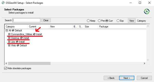
- Next click the circle to select install for: commandline_Utilities, Desktop, and Libs
R and RStudio
In order to utilize RStudio we first need to download R. This can be downloaded for Windows from https://cran.r-project.org/bin/windows/base/. For this installer we will be accepting all of the default paths and options.
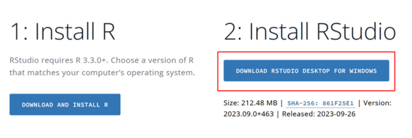
Now we can download RStudio, similar to R we will be utilizing all default paths and options. RStudio can be downloaded here. At the time of writing RStudio version 2023.09.0+463 is the most current update, and requires an R installation of 3.3.0+ or above.
RStudio setup
Now that we have all of the software that we need we can proceed with setting up RQGIS within RStudio. In order to run QGIS functions within RStudio we will need to download and unpack some packages which allow for the manipulation of spatial data. After installing these packages within the workspace we will link our workspace with the root directory of QGIS in order to gain access to its host of functions and algorithms.
Install Packages
Start by opening up RStudio and creating a new ‘’’R script’’’ file (file->new file->R script). Within this new script we will be downloading and installing some packages that allow us to manipulate raster and spatial data within RStudio. Start by adding this code to your script and running it.
#Install packages
install.packages("sp")
install.packages("sf")
install.packages("geodata")
install.packages("qgisprocess")
install.packages("raster")
install.packages("rgdal")
#Attach packages to workspace
library("sp")
library("sf")
library("geodata")
library("qgisprocess")
library("raster")
library("rgdal")
- sp: provides functions for plotting spatial data
- sf: provides functions for using spatial features
- geodata: provides open source spatial data used in the tutorial
- qgisprocess: Creates a link between the IDE (RStudio) and functions found within QGIS
- raster: Provides the user to read, write and manipulate raster images within RStudio
- rgdal: Provides the user to read, write and manipulate shapefiles within RStudio
Data Acquisition
In this tutorial we will make use of datasets that are accessible within RStudio as a method of showcasing the use of various QGIS geoprocessing functions. In order to access these datasets you use the data() function which provides the user with a list of all available datasets preloaded within RStudio. Additionally, the getData() function allows the user to download geographic data for specific countries around the world.
Setting Path
First we will make sure the working directory is set to the C: drive of your computer. This can be done using the setwd("C:") command which will ensure all path based commands use the root C: directory as their base. You can also use this command to set the working directory for R as a different folder location, however this may cause problems if you have spaces in your file paths so use with caution. Additionally, we will make a variable called path which will point to the location that we want and input/output files to be stored. This path will then be used in subsequent commands by adding concatenating the string variable of the path with the name of the file, such as paste(path,"/output.txt", sep="")).
#Create a working directory for this tutorial
setwd("C:")
path = "C:/Users/razzroutly/Documents/Classes/GEOM4008"
Importing Data
One of the advantages of using RStudio as an alternative GIS is its ability to load open source geospatial data with just one line of code. For this tutorial we will be using the geodata package to access digital elevation models using the elevation_30s() command which will provide a raster with 30 arc second (1km) from the Shuttle Radar Topography Mission, supplemented by GTOP30 data for high latitudes [1].
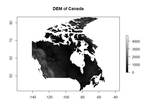
We will import the dataset that used in this tutorial into our workspace and display it within the RStudio plot frame. We will be downloading a DEM of Canada from the geodata package. The getData() function downloads data from an online database. Due to the high resolution of the raster we will also use a function from the raster package that will aggregate the raster cells by a factor of 10 to make processing easier.
#Digital elevation model (DEM) of Canada
canada_dem<-getData('alt', country='CAN', mask=TRUE)
plot(canada_dem, col=grey(0:100/100), main='DEM of Canada')
canada_dem_agg <- aggregate(canada_dem, fact=10)
After running this code you will notice that the DEM's are displayed in the lower right plot window. The outputs should look like this:
.
QGIS Functions
In order to utilize QGIS functions within RStudio, we first have to learn how to find the functions we want to use with their respective syntax, as well as learn what parameters we will be working with for each function. In order to do this we will be making use of the qgis_search_algorithms() and qgis_show_help() functions. The qgis_search_algorithms() function allows the user to enter a keyword for the function they are interested in using, and provides the user with a list of available functions that pertain to that keyword as well as which provider within QGIS they come from (SAGA, GDAL, GRASS, etc.), algorithims that are found in the base version of QGIS have the provider "native". After selecting the function that we are interested in using we can use the qgis_show_help() function to display a description of the use for the function as well as the input and output parameters that the function utilizes. As an example we will use the qgis_search_algorithms() function to search for a clipping function.
#Searches for functions which contain the keyword 'clip'
qgis_search_algorithms(algorithm="clip")
After running this line you will see a list of 11 clipping tools that have been displayed in the console.
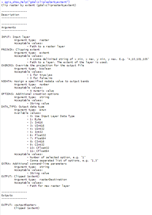
We will select the GDAL clipping function gdal:cliprasterbyextent and determine which parameters we will need to be able to make use of this function in RStudio. To do this we will use the qgis_get_argument_specs() function. In order to use this function we need to use the full name of the function which is gdal:cliprasterbyextent.
#Provides the user with information regarding the parameters of a function
qgis_show_help("gdal:cliprasterbyextent")
When running this line of code you will see a list of the functions parameters appear in the console. This provides you with information regarding the type of input required for each parameter and provides the user with a legend for parameters that are normally accessed through drop down boxes in QGIS.
Now that we know how to search for the functions we would like to use we can go on to utilize these functions to analyze DEM files.
Raster to Vector
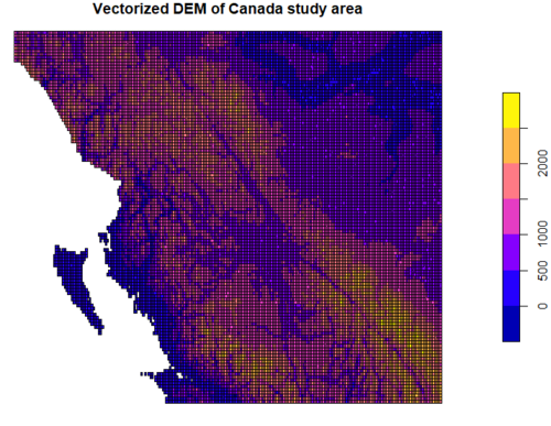
The first algorithm we will investigate is gdal:polygonize. This algorithm takes a raster image and converts its features into polygons. In order to use this function we will need to determine the parameters for: input, field, and output. The qgis_run_algorithm() function takes in the desired algorithm as well as that algorithms parameters, since the output of this function is very large we will be storing the output vector in the temporary files of qgisprocess. This is done leaving out the OUTPUT parameter within the arguments and then calling the st_as_sf() function on the result of the algorithim.
#Conversion of DEM to shapefile format
output <- qgis_run_algorithm("gdal:polygonize", INPUT=canada_dem_clip, FIELD="values", BAND=1)
canada_poly <- st_as_sf(output)
plot(canada_poly)
After running this code you will see a vector interpretation of the clipped study area. Here is a side by side comparison between the DEM and its shapefile counterpart.
.
Clipping
Raster Clipping
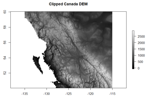
In order to clip raster files we will make use of the gdal:cliprasterbyextent algorithm. This algorithm takes in a raster input, the desired clipping extent, output raster type and the desired output raster file. Additionally, I have provided a clipping extent for the image so that we can test this algorithm.
#Clipped version of the original Canada DEM
qgis_run_algorithm("gdal:cliprasterbyextent", INPUT=canada_dem, PROJWIN = "-135,-115,50,60", OUTPUT=paste(path,"/clip_dem.tif", sep=""))
canada_dem_clip<-raster(paste(path,"/clip_dem.tif", sep=""))
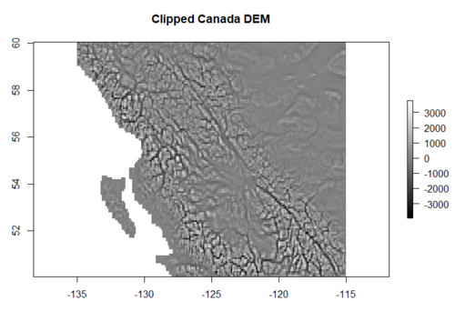
plot(canada_dem_clip,col=grey(0:100/100), main='Clipped Canada DEM')
After running this function we plot the raster image, the result should represent the section of Canada that we specified as the extent in the algorithm.
Raster to Vector
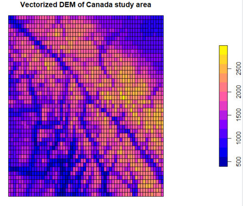
To demonstrate using clipping algorithms on vector files we will first need to change the raster of the Canada DEM to a vector using the GDAL polygonize algorithm which takes a raster image and converts its features into polygons. In order to use this function we will need to determine the parameters for: input, field, and output using the qgis_show_help() function. Since the output of this function is very large we will be storing the output vector in the temporary files of qgisprocess. This is done by leaving out the OUTPUT parameter causing it to default to qgis_temp_vector() and then calling the st_as_sf() function on the result of the algorithm.
#Conversion of DEM to shapefile format
qgis_show_help("gdal:polygonize")
output <- qgis_run_algorithm("gdal:polygonize", INPUT=canada_dem_clip, FIELD="values", BAND=1)
canada_poly <- st_as_sf(output)
plot(canada_poly)
After running this code you will see a vector interpretation of the clipped study area. Here is a side by side comparison between the DEM and its shapefile counterpart.
Vector clipping
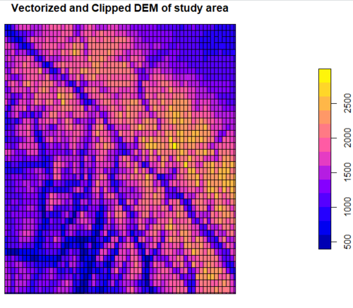
To demonstrate clipping vector data using qgisprocess we will now further clip down the British Columbia study area using the gdal:clipvectorbyextent algorithm. This algorithm takes the vector shapefile as an input, a specified clipping extent, and a specified output for the result. Try running the code provided below.
#Take an input shapefile and clip it to the specified extent
poly_output <- qgis_run_algorithm("gdal:clipvectorbyextent", INPUT=canada_poly, EXTENT = "-121,-116,50.2,53.8")
vector_clip <- st_as_sf(poly_output)
plot(vector_clip, main='Vectorized and Clipped DEM of study area')
The result of the shapefile clip should display the shapefile that has been clipped to the extent specified within the qgis_run_algorithm function.
Laplacian Filter
In this example we will utilize a Laplacian filter on the clipped raster version of the Canadian DEM. The Laplacian filter will be used to highlight the edges of the mountain range and gullies. To utilize a Laplacian filter within RStudio we will use a SAGA algorithm found within QGIS, saga:laplacianfilter. In order to use the Laplacian filter we need an input raster, kernel method and type, radius, and sampling method. The code to run this filter on the clipped version of the Canadian DEM is provided below.
#Creates a new raster image depicting the filtered Canadian DEM
qgis_run_algorithm("saga:laplacianfilter", INPUT=canada_dem_clip, METHOD = 2, KERNEL_RADIUS = 1, KERNEL_TYPE = 0, RESULT=paste(path,"/laplacian.tif", sep=""))
lap_output<-raster(paste(path,"/laplacian.tif", sep=""))
plot(lap_output,col=grey(0:100/100), main='Clipped Canada DEM')
The resulting output is a filtered version of the original DEM. The Laplacian filter is often used for edge detection and is useful for analyzing mountain ranges as shown below.
Hillshade
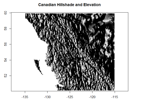
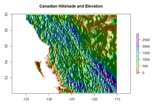
The hillshade function creates a 3D representation of the original DEM. This function is available within RStudio and is called gdal:hillshade. In order to use this function we will need to set the azimuth angle and slope, we will use 270 and 40 degrees respectively. Hillshade analysis is useful for generating 3D images representative of the DEM plot. First we will create a hillshade raster with the gdal:hillshade algorithm, then we will overlay the original DEM to provide elevation as additional context to the image.
#Hillshade function applied to the Canadian DEM, overlain by the original DEM
qgis_run_algorithm("gdal:hillshade", INPUT=canada_dem_clip, AZIMUTH = 270, ALTITUDE=40, OUTPUT=paste(path,"/hillshade.tif", sep=""))
hillshade<-raster(paste(path,"/hillshade.tif", sep=""))
plot(hillshade, col=grey(0:100/100), legend=FALSE, main='Canadian Hillshade and Elevation')
plot(canada_dem_clip, col=rainbow(25, alpha=0.35), add=TRUE)
Below you can see the output generated from the hillshade as well as the output generated by overlaying the DEM.
.
Conclusion
After finishing this tutorial my hope is that the user will have a functional workspace within RStudio in which they can utilize the various functions demonstrated. Additionally, I believe I have provided the tools necessary for users to explore and search for algorithms that they may need to use within their own projects. RStudio provides a unique environment for the user to create custom scripts to manage QGIS geoprocessing algorithms.

