Difference between revisions of "Evaluating Landscape Permeability in Quantum"
m (→Disclaimer) |
|||
| (95 intermediate revisions by one other user not shown) | |||
| Line 1: | Line 1: | ||
==Disclaimer== |
==Disclaimer== |
||
::[[File: |
::[[File:animation.gif|thumb|100px|frame| Vancouver Island Grey Wolf]] |
||
Please note that this Wiki has been produced for the [http://www4.carleton.ca/cu0809uc/courses/GEOM/4008.html GEOM4008 Advanced Topics in Geographic Information Systems] class at [http://carleton.ca/ Carleton University] strictly as a tutorial to showcase the method of calculating landscape permeability using FOSS. The results should by no means be taken as a true analysis of grey wolf movement since much of the data |
Please note that this Wiki has been produced for the [http://www4.carleton.ca/cu0809uc/courses/GEOM/4008.html GEOM4008 Advanced Topics in Geographic Information Systems] class at [http://carleton.ca/ Carleton University] strictly as a tutorial to showcase the method of calculating landscape permeability using FOSS. The results should by no means be taken as a true analysis of grey wolf movement since much of the data were fictional. |
||
==Introduction== |
==Introduction== |
||
The objective of this project was to develop a method to evaluate landscape permeability for large carnivores using only [http://en.wikipedia.org/wiki/Free_and_open-source_software Free and Open-Source Software (FOSS)]. This tutorial has been created to allow non-GIS individuals to successfully complete this analysis in Quantum GIS (1.7.4) using the |
The objective of this project was to develop a method to evaluate [http://www.rewilding.org/LandscapePermeability.html landscape permeability] for large carnivores using only [http://en.wikipedia.org/wiki/Free_and_open-source_software Free and Open-Source Software (FOSS)]. This tutorial has been created to allow non-GIS individuals to successfully complete this analysis in [http://www.qgis.org/ Quantum GIS] (1.7.4) using the [http://grass.osgeo.org/ GRASS] Plugin. This tutorial will be carried out while analyzing the landscape permeability for grey wolf movement on [http://en.wikipedia.org/wiki/Vancouver_Island Vancouver Island]. The final result of this project will be a landscape permeability map which will attempt to provide valuable insight into the movement of the [http://www.geog.uvic.ca/viwilds/iw-wolf.html Vancouver Island grey wolf]. This sort of information could potentially be used to implement more successful conservation strategies, facilitate [http://en.wikipedia.org/wiki/Ecosystem-based_management ecosystem-based management] (EBM), and better understand the genetic flow of the island’s population. |
||
==Data== |
==Data== |
||
| Line 15: | Line 16: | ||
|+'''Table 1. Data Used and Data Sources for Vancouver Island Grey Wolf''' |
|+'''Table 1. Data Used and Data Sources for Vancouver Island Grey Wolf''' |
||
|- |
|- |
||
! style="background:# |
! style="color:#FFFFFF; background:#228822;" | Data Used |
||
! style="background:# |
! style="color:#FFFFFF; background:#228822;" | Data Format |
||
! style="background:# |
! style="color:#FFFFFF; background:#228822;" | Data Source |
||
|- |
|- |
||
| Boundary of Vancouver Island |
| Boundary of Vancouver Island |
||
| Line 33: | Line 34: | ||
| Landcover |
| Landcover |
||
| Vector Polygon |
| Vector Polygon |
||
| [http://www.geobase.ca/geobase/en/data/landcover/index.html;jsessionid=8AA56CB430A0F096D082E9FEFC70C3EC GeoBase] Layer: Land Cover / |
| [http://www.geobase.ca/geobase/en/data/landcover/index.html;jsessionid=8AA56CB430A0F096D082E9FEFC70C3EC GeoBase] Layer: Land Cover / Circa 2000 |
||
|- |
|- |
||
| DEM |
| DEM |
||
| Line 61: | Line 62: | ||
==Methods== |
==Methods== |
||
It is highly recommended that these methods are done in order |
It is highly recommended that these methods are done in sequential order due to the number of step needed to complete this analysis. |
||
===QGIS Setup=== |
===QGIS Setup=== |
||
| Line 71: | Line 72: | ||
===Opening QGIS=== |
===Opening QGIS=== |
||
Before beginning, ensure that Quantum GIS is installed on the computer you wish to use. If you do not have QGIS installed, [http://hub.qgis.org/projects/quantum-gis/wiki/Download download QGIS]. |
Before beginning, ensure that Quantum GIS is installed on the computer you wish to use. If you do not have QGIS installed, [http://hub.qgis.org/projects/quantum-gis/wiki/Download download QGIS]. |
||
*Once the installation has been completed, or if QGIS was already installed, click the QGIS |
*Once the installation has been completed, or if QGIS was already installed, click the QGIS Icon to open the program. [[File:Icon.png]] This will open the initial QGIS Window. |
||
*Immediately go to the File Tab. [[File:Filetab.png]] |
*Immediately go to the File Tab. [[File:Filetab.png]] |
||
*Click Save Project As. [[File:Saveas.png]] |
*Click Save Project As. [[File:Saveas.png]] |
||
*Save your project in the folder with all your data. |
*Save your project in the folder with all your data. |
||
*IMPORTANT NOTE: Remember to save your project often. [[File:Save.png]] |
*IMPORTANT NOTE: Remember to save your project often by clicking Save. [[File:Save.png]] |
||
===Installing the |
===Installing the GRASS Plugin=== |
||
Once the initial QGIS window has been opened, it is highly recommended that the GRASS |
Once the initial QGIS window has been opened, it is highly recommended that the GRASS Plugin be installed next. The GRASS Plugin allows the tools from [http://grass.osgeo.org/ GRASS GIS] to be used within QGIS. |
||
*Go to the Plugins Tab. [[File:Pluginstab.png]] |
*Go to the Plugins Tab. [[File:Pluginstab.png]] |
||
*Click Manage Plugins. [[File:Manageplugins.png]] |
*Click Manage Plugins. [[File:Manageplugins.png]] |
||
*This will bring you to the QGIS Plugin Manager Window. |
*This will bring you to the QGIS Plugin Manager Window. |
||
*In filter write GRASS. [[File:filterg.png]] |
*In filter write GRASS. [[File:filterg.png]] |
||
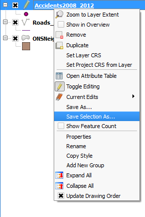
*Click on the GRASS Plugin and make sure there is an |
*Click on the GRASS Plugin and make sure there is an X in the box. [[File:GRASS.png]] |
||
*Finally, click OK. [[File:OK.png]] |
*Finally, click OK. [[File:OK.png]] |
||
*Now, go back to the Plugins Tab, [[File:Plugins.png]] a new GRASS Tab should have appeared. [[File:GRASS1.png]] |
*Now, go back to the Plugins Tab, [[File:Plugins.png]] a new GRASS Tab should have appeared. [[File:GRASS1.png]] |
||
*Expanding this GRASS menu reveals that most of the tools are greyed out. |
*Expanding this GRASS menu reveals that most of the tools are greyed out. |
||
*In order to fix this click on New Mapset. The Mapset is the location where you want your |
*In order to fix this click on New Mapset. The Mapset is the location where you want your GRASS files to be stored. [[File:NewMapset.png]] |
||
*Click Browse [[File:Browse.png]], and then go to your chosen destination. |
*Click Browse [[File:Browse.png]], and then go to your chosen destination. |
||
*Once you have browsed to the location, click Next. [[File:Next.png]] |
*Once you have browsed to the location, click Next. [[File:Next.png]] |
||
*Now you will create a new GRASS location. We named ours GRASS. [[File:Newlocation.png]] |
*Now you will create a new GRASS location. We named ours GRASS. [[File:Newlocation.png]] |
||
*Then click Next. [[File:Next.png]] |
*Then click Next. [[File:Next.png]] |
||
*This will bring you to the Projection |
*This will bring you to the Projection Window. Defining your projection is extremely important. |
||
*Click the circle beside Projection. [[File:Projection.png]] You must chosen the projection based on your study location; for more information on choosing an appropriate projection, see this [http://www.georeference.org/doc/guide_to_selecting_map_projections.htm Guide to Selecting Map Projections]. Since our location was in Vancouver Island, we chose Universal |
*Click the circle beside Projection. [[File:Projection.png]] You must chosen the projection based on your study location; for more information on choosing an appropriate projection, see this [http://www.georeference.org/doc/guide_to_selecting_map_projections.htm Guide to Selecting Map Projections]. Since our location was in Vancouver Island, we chose Universal Transverse Mercator (UTM), NAD83 (NSRS2007) /UTM zone 10N. [[File:Zone10.png]] |
||
*Once you have chosen your |
*Once you have chosen your Projection, click Next. [[File:Next.png]] |
||
*This will bring you to the Define GRASS Region Window. |
*This will bring you to the Define GRASS Region Window. |
||
*Scroll to the country of your study area, and click Set. [[File:Set.png]] |
*Scroll to the country of your study area, and click Set. [[File:Set.png]] |
||
*Then click Next. [[File:Next.png]] |
*Then click Next. [[File:Next.png]] |
||
*This will bring you to the Mapset |
*This will bring you to the Mapset Window. |
||
*Name your new Mapset. We named ours Mapset. [[File:Mapset.png]] |
*Name your new Mapset. We named ours Mapset. [[File:Mapset.png]] |
||
*Click Next. [[File:Next.png]] |
*Click Next. [[File:Next.png]] |
||
| Line 109: | Line 110: | ||
==Workspace Setup== |
==Workspace Setup== |
||
Before beginning any data processing, the |
Before beginning any data processing, the data must be added and the region must be set up. |
||
===Adding Vector Layers to QGIS=== |
===Adding Vector Layers to QGIS=== |
||
*To add vector layers, click the |
*To add vector layers, click the Add Vectors layer button at the top left of the screen. [[File:Addveclayer.png]] |
||
*Browse to the location where you saved your data. [[File:Browse.png]] |
*Browse to the location where you saved your data. [[File:Browse.png]] |
||
*Click Open. [[File:Open.png]] |
*Click Open. [[File:Open.png]] |
||
| Line 122: | Line 123: | ||
*Navigate to the desired folder using the Browse button. [[File:Browse.png]] |
*Navigate to the desired folder using the Browse button. [[File:Browse.png]] |
||
*Chose the w001001.adf file. |
*Chose the w001001.adf file. |
||
*Then click Open. [[File:Open.png]] These layers will show up in the TOC on the left. The raster layers we added to the project included: Road Density and |
*Then click Open. [[File:Open.png]] These layers will show up in the TOC on the left. The raster layers we added to the project included: Road Density and the DEM. |
||
*In the TOC, right click on the layer that says w001001. [[File:w001001.png]] |
*In the TOC, right click on the layer that says w001001. [[File:w001001.png]] |
||
*Click on |
*Click on Properties. [[File:Properties.png]] |
||
*Within the |
*Within the Layer Properties, go to the General Tab. [[File:General.png]] |
||
*Under Display Name, give the layer an appropriate name. |
*Under Display Name, give the layer an appropriate name. For example, DEM. [[File:Displayname.png]] |
||
*Next, go to the Style Tab. [[File:Style.png]] |
*Next, go to the Style Tab. [[File:Style.png]] |
||
*Change the Color Map option to be Pseudocolour. [[File:Pseudocolor.png]] |
*Change the Color Map option to be Pseudocolour. [[File:Pseudocolor.png]] |
||
*Then click OK. [[File:OK.png]] |
*Then click OK. [[File:OK.png]] |
||
===Editing the Current |
===Editing the Current GRASS Region=== |
||
It is very important to edit the Current GRASS Region in order to specify the processing extents and resolution. |
It is very important to edit the Current GRASS Region in order to specify the processing extents and resolution. |
||
*To do this, go to the Plugins Tab. [[File:Plugins.png]] |
*To do this, go to the Plugins Tab. [[File:Plugins.png]] |
||
| Line 137: | Line 138: | ||
*Then click the Edit Current GRASS Region Button. [[File:Region.png]] |
*Then click the Edit Current GRASS Region Button. [[File:Region.png]] |
||
*The extent can be created by drawing an area of interest around your boundary layer. |
*The extent can be created by drawing an area of interest around your boundary layer. |
||
*Next the resolution must be changed. Change the cell width and cell height. We changed our cell width and height to be 50. This may be dependent on your data. Originally we tried a cell size of 90; however, this produced images that were too course. We also tried a a cell size of 10; however, this would not run. |
|||
* |
*After you have changed the cell size click OK. [[File:OK.png]] |
||
==Data Processing== |
==Data Processing== |
||
The data processing steps will set up all your layers in the proper formats to be used in the landscape permeability evaluation. |
The data processing steps will set up all your layers in the proper formats to be used in the landscape permeability evaluation. |
||
===Clipping Vector Layers to AOI boundary=== |
===Clipping Vector Layers to AOI boundary=== |
||
*To clip all the layers to your Area of Interest (AOI), go to the Vector Tab. [[File:Vectortab.png]] Ex. we used the Vancouver Island boundary files as our AOI. |
*To clip all the layers to your Area of Interest (AOI), go to the Vector Tab. [[File:Vectortab.png]] Ex. we used the Vancouver Island boundary files as our AOI. |
||
*Click Geoprocessing Tools. [[File:Geoprocessing.png]] |
*Click Geoprocessing Tools. [[File:Geoprocessing.png]] |
||
*Then click Clip. [[File:Clip.png]] |
*Then click Clip. [[File:Clip.png]] |
||
*The |
*The input vector layer is the layer that needs to be clipped. [[File:Roads.png]] For example we had to clip our Roads file which originally contained all the Roads in BC. |
||
*The Clip layer is the layer you wish to be your AOI. [[File:cliplayer.png]] |
*The Clip layer is the layer you wish to be your AOI. [[File:cliplayer.png]] |
||
*Name the output shapefile and specify an appropriate location for it. [[File:browse.png]] |
*Name the output shapefile and specify an appropriate location for it. [[File:browse.png]] |
||
| Line 164: | Line 167: | ||
===Editing the Attribute Table=== |
===Editing the Attribute Table=== |
||
The attribute table must be edited on all the layers you preformed a union on |
The attribute table must be edited on all the layers you preformed a union on. A CLASS field will house the unique values from which we will create our rasters later on. |
||
*To open the attribute table, right click on the layer. [[File:Openatttable.png]] |
*To open the attribute table, right click on the layer. [[File:Openatttable.png]] |
||
*Left click on Open Attribute Table. |
*Left click on Open Attribute Table. |
||
*In order to edit, click the |
*In order to edit, click the Editor Mode on. [[File:Edit.png]] |
||
*Create a new column by clicking New Column. [[File:Newcolumn.png]] |
*Create a new column by clicking New Column. [[File:Newcolumn.png]] |
||
*The |
*The Add Column Window will pop up. Give the column a name. We named our CLASS. [[File:Columnname.png]] |
||
*If you would like, you can give the column a comment; however, it is not necessary. |
*If you would like, you can give the column a comment; however, it is not necessary. |
||
*Ensure the type is set to whole number (integer), [[File:type.png]] with a width of 1. [[File:width.png]] |
*Ensure the type is set to whole number (integer), [[File:type.png]] with a width of 1. [[File:width.png]] |
||
| Line 177: | Line 180: | ||
*As you click the numbers, sections of the map will become highlighted. [[File:Highlight.png]] |
*As you click the numbers, sections of the map will become highlighted. [[File:Highlight.png]] |
||
*Again, once you have found the boundary, put a 1 in the CLASS column and a 2 in the rest of the columns. |
*Again, once you have found the boundary, put a 1 in the CLASS column and a 2 in the rest of the columns. |
||
*To save changes click the |
*To save changes click the Editor Mode button again. [[File:Edit.png]] |
||
===Importing Vectors to |
===Importing Vectors to GRASS Format=== |
||
To use the GRASS |
To use the GRASS Plugin all the layers must be imported into a GRASS format. For all the vector layers the tool v.in.ogr.qgis must be used. |
||
*To do so go to the Plugins Tab. [[File:Plugins.png]] |
*To do so go to the Plugins Tab. [[File:Plugins.png]] |
||
*Click |
*Click GRASS. [[File:GRASS1.png]] |
||
*Then click Open GRASS Tools. [[File:Grasstools.png]] |
*Then click Open GRASS Tools. [[File:Grasstools.png]] |
||
*Next go to the Modules List Tab. [[File:Moduleslist.png]] |
*Next go to the Modules List Tab. [[File:Moduleslist.png]] |
||
*In the |
*In the Filter Box type v.in.ogr.qgis. [[File:filterv.png]] |
||
*Click on the Correct Tool. [[File:grassvec.png]] |
*Click on the Correct Tool. [[File:grassvec.png]] |
||
*The tool will pop up. |
*The tool will pop up. |
||
*Use the drop down OGR vector layer arrow to select a layer to change to |
*Use the drop down OGR vector layer arrow to select a layer to change to GRASS format. [[File:vectlayer.png]] |
||
*IMPORTANT NOTE: the layer must be on in the |
*IMPORTANT NOTE: the layer must be on in the TOC for the drop down to function. |
||
*Give the |
*Give the Output Vector Map a name. [[File:outputvec.png]] An example of our naming scheme is Deforest_U_G, where the "G" signifies that it is now in a GRASS vector format. |
||
*Click Run. [[File:Run.png]] |
*Click Run. [[File:Run.png]] |
||
*Once the tool has successfully finished, click View Output. [[File:ViewOutput.png]] The layer will appear in the TOC. |
*Once the tool has successfully finished, click View Output. [[File:ViewOutput.png]] The layer will appear in the TOC. |
||
===Importing Rasters to |
===Importing Rasters to GRASS Format=== |
||
To use the GRASS |
To use the GRASS Plugin, all the raster layers must also be imported into a GRASS format. For all the raster layers the tool r.in.gdal.qgis must be used. |
||
*To do this, go to the Plugins Tab. [[File:Plugins.png]] |
*To do this, go to the Plugins Tab. [[File:Plugins.png]] |
||
*Click |
*Click GRASS. [[File:GRASS1.png]] |
||
*Then click Open GRASS Tools. [[File:Grasstools.png]] |
*Then click Open GRASS Tools. [[File:Grasstools.png]] |
||
*Go to the Modules List Tab. [[File:Moduleslist.png]] |
*Go to the Modules List Tab. [[File:Moduleslist.png]] |
||
*In the |
*In the Filter Box, type r.in.gdal.qgis. [[File:filterr.png]] |
||
*Click on the correct tool. [[File:grassras.png]] |
*Click on the correct tool. [[File:grassras.png]] |
||
*The tool will popup. |
*The tool will popup. |
||
*Use the drop down loaded layer arrow to select a layer to change to |
*Use the drop down loaded layer arrow to select a layer to change to GRASS format. [[File:grassrasinput.png]] |
||
*IMPORTANT NOTE: the layer must be on in the TOC and activated it show up in the dropdown menu. |
*IMPORTANT NOTE: the layer must be on in the TOC and activated it show up in the dropdown menu. |
||
*Give the |
*Give the Output Raster Map a name a click Run. [[File:Run.png]] An example of our naming scheme is DEM_G. [[File:grassrasoutput2.png]] |
||
*Once the tool has successfully finished, click View Output. [[File:ViewOutput.png]] The layer will appear in the TOC. |
*Once the tool has successfully finished, click View Output. [[File:ViewOutput.png]] The layer will appear in the TOC. |
||
| Line 214: | Line 217: | ||
*Then click Open GRASS Tools. [[File:Grasstools.png]] |
*Then click Open GRASS Tools. [[File:Grasstools.png]] |
||
*Go to the Modules List. [[File:Moduleslist.png]] |
*Go to the Modules List. [[File:Moduleslist.png]] |
||
*In the |
*In the Filter Box, type in v.to.rast.attr. [[File:filterv.to.r.png]] |
||
*Click on the correct tool. [[File:v.to.rast.png]] and the tool will then open. |
*Click on the correct tool. [[File:v.to.rast.png]] and the tool will then open. |
||
*Using the dropdown menu, select input vector layer you wish to rasterize. [[File:inputv.to.r.png]] |
*Using the dropdown menu, select input vector layer you wish to rasterize. [[File:inputv.to.r.png]] |
||
*Remember, the layer must be on for it to appear in the dropdown menu. |
*Remember, the layer must be on for it to appear in the dropdown menu. |
||
*In the Attribute |
*In the Attribute Field, select the CLASS layer that you created. [[File:attclass.png]] |
||
*Give the |
*Give the Output Raster Map a name. [[File:v.to.routput.png]] |
||
*Click Run. [[File:Run.png]] |
*Click Run. [[File:Run.png]] |
||
*Finally, click View Output. [[File:ViewOutput.png]] |
*Finally, click View Output. [[File:ViewOutput.png]] |
||
===Raster Data Processing: Creating the Slope Layer=== |
===Raster Data Processing: Creating the Slope Layer=== |
||
To create a |
To create a Slope layer, a Digital Elevation Model (DEM) must be given as the input. |
||
*Go to the Plugins Tab. [[File:Plugins.png]] |
*Go to the Plugins Tab. [[File:Plugins.png]] |
||
*Click |
*Click GRASS. [[File:GRASS1.png]] |
||
*Click Open |
*Click Open GRASS Tools. [[File:Grasstools.png]] |
||
*Go to the Modules List. [[File:Moduleslist.png]] |
*Go to the Modules List. [[File:Moduleslist.png]] |
||
*In the |
*In the Filter Box, type Slope. [[File:Filterslope.png]] |
||
*Click the Slope Tool. [[File:Slope.G.png]] |
*Click the Slope Tool. [[File:Slope.G.png]] |
||
*Input the name of the |
*Input the name of the Elevation Raster Map (DEM). [[File:slopeinput.png]] |
||
*Name the |
*Name the Output Slope Raster Map. Our output map was named Slope. [[File:slopeoutput.png]] |
||
*The format for reporting the slope can be degrees or percent; we used degrees. [[File:Degrees.png]] |
*The format for reporting the slope can be degrees or percent; we used degrees. [[File:Degrees.png]] |
||
*Click Run. [[File:Run.png]] |
*Click Run. [[File:Run.png]] |
||
| Line 247: | Line 250: | ||
[[File:Reclassrules.png]] |
[[File:Reclassrules.png]] |
||
*In the image shown above, the first column on the left indicates each unique pixel value in the raster (recall, for the layers in which a union was required,these values would be 1 (the boundary) and 2 (ex.lakes)). The second column indicates the cost value you wish to reassign to each pixel. |
*In the image shown above, the first column on the left indicates each unique pixel value in the raster (recall, for the layers in which a union was required,these values would be 1 (the boundary) and 2 (ex.lakes)). The second column indicates the cost value you wish to reassign to each pixel. |
||
*If the raster has more than two unique values, then you can assign a single cost value to a range of slope values. This example is demonstrated below using our Slope |
*If the raster has more than two unique values, then you can assign a single cost value to a range of slope values. This example is demonstrated below using our Slope Raster. |
||
[[File:reclassrulesslope.png]] |
[[File:reclassrulesslope.png]] |
||
*For further help creating the reclass rule files see [http://grass.osgeo.org/grass64/manuals/r.reclass.html r.reclass |
*For further help creating the reclass rule files see [http://grass.osgeo.org/grass64/manuals/r.reclass.html r.reclass GRASS Help] |
||
===Running the Reclass Tool=== |
===Running the Reclass Tool=== |
||
| Line 257: | Line 260: | ||
*Click Open GRASS Tools. [[File:Grasstools.png]] |
*Click Open GRASS Tools. [[File:Grasstools.png]] |
||
*Go to the Modules List. [[File:Moduleslist.png]] |
*Go to the Modules List. [[File:Moduleslist.png]] |
||
*In the |
*In the Filter Box, type in r.reclass. [[File:filterreclass.png]] |
||
*Click on the correct tool. [[File:r.reclass.png]] |
*Click on the correct tool. [[File:r.reclass.png]] |
||
*Input the raster map to be reclassified. [[File:reclasinput.png]] |
*Input the raster map to be reclassified. [[File:reclasinput.png]] |
||
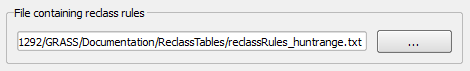
*For the File Containing Reclass Rules parameter, |
*For the File Containing Reclass Rules parameter, Browse to the location of your saved reclass rules text file. [[File:reclassrulesinput.png]] |
||
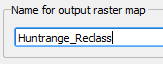
*Specify an |
*Specify an Output Raster Map name. For example we called ours Huntrange_Reclass. [[File:relcassoutput.png]] |
||
*Now click Run. [[File:Run.png]] |
*Now click Run. [[File:Run.png]] |
||
*Then, click View Output. [[File:ViewOutput.png]] |
*Then, click View Output. [[File:ViewOutput.png]] |
||
===Combining the Cost Rasters in the Map Calculator=== |
===Combining the Cost Rasters in the Map Calculator=== |
||
To create a cost raster that displays the cumulative cost of moving over the land, all the individual cost rasters must be added together using the |
To create a cost raster that displays the cumulative cost of moving over the land, all the individual cost rasters must be added together using the Raster Map Calculator. |
||
*Go to the Plugins Tab. [[File:Plugins.png]] |
*Go to the Plugins Tab. [[File:Plugins.png]] |
||
*Click GRASS. [[File:GRASS1.png]] |
*Click GRASS. [[File:GRASS1.png]] |
||
*Click Open GRASS Tools. [[File:Grasstools.png]] |
*Click Open GRASS Tools. [[File:Grasstools.png]] |
||
*Go to the Modules List. [[File:Moduleslist.png]] |
*Go to the Modules List. [[File:Moduleslist.png]] |
||
*In the |
*In the Filter Box, type in r.mapcalculator. [[File:filtermapcalc.png]] |
||
*Click on the map calculator tool. [[File:r.mapcalc.png]] |
*Click on the map calculator tool. [[File:r.mapcalc.png]] |
||
[[File:Picture1005.png]] |
[[File:Picture1005.png]] |
||
| Line 287: | Line 290: | ||
Before starting the actual evaluation, look at Figure 5 below. This shows the locations of the fictitious wolf ranges (i.e. areas where metapopulations of wolves are known to reside). The ranges are labeled A through D, from North to South, respectively. The goal of this analysis was to identify which paths pose the least resistant/danger to movement between each of these ranges. |
Before starting the actual evaluation, look at Figure 5 below. This shows the locations of the fictitious wolf ranges (i.e. areas where metapopulations of wolves are known to reside). The ranges are labeled A through D, from North to South, respectively. The goal of this analysis was to identify which paths pose the least resistant/danger to movement between each of these ranges. |
||
[[File:boundarypoints2.png]] ::[[File:wolf3.png|thumb|100px|frame| Grey Wolf]] |
|||
[[File:boundarypoints2.png]] |
|||
'' Figure 5: The location of wolf ranges A, B, C, and D. '' |
'' Figure 5: The location of wolf ranges A, B, C, and D. '' |
||
| Line 302: | Line 301: | ||
===Generating an Accumulated Cost Surface using r.walk=== |
===Generating an Accumulated Cost Surface using r.walk=== |
||
The r.walk.vect tool creates |
The r.walk.vect tool creates an accumulative cost distance value for each cell compared to the specified source location. This means that cells farther from the source feature will receive a higher cost distance value than cells closer to the source feature. This accumulated cost distance surface is a required input of the r.drain tool which actually generates the least cost path. In our example we wanted to inspect the path from wolf range A to D, so location A would be the starting point. |
||
*Go to the Plugins Tab. [[File:Plugins.png]] |
*Go to the Plugins Tab. [[File:Plugins.png]] |
||
| Line 392: | Line 391: | ||
==Conclusion== |
==Conclusion== |
||
Repeating the r.walk and r.drain processes of creating least cost paths and corridors for each combination of starting and ending destinations (AB,AC,AD,BC,BD,CD). You can create a map that resembles Figure 10 by turning on all these created layers in the TOC. This map shows all the possible least cost paths to each wolf range overlaid on an cumulative least cost corridor. This cumulative least cost corridor was created by adding all of the accumulated cost surfaces for each starting point together, as shown in Figure 11. Sometimes, it might be appropriate to overlay the paths on other surfaces, such as the master cost raster (e.g. Figure 12). This map just emphasizes that the paths in actual fact do follow the least costly (lighter cells) routes. For example, the large whiter circles represent the radius around the hunt camps, which were assigned a cost factor of 9; as a result, the paths serve around all of these dangerous areas. |
|||
[[File:coridoor&path2.png]] |
[[File:coridoor&path2.png]] |
||
'' Figure 10: (Above) The final map showing all the possible least cost paths to each wolf range overlaid on |
'' Figure 10: (Above) The final map showing all the possible least cost paths to each wolf range overlaid on a cumulative least cost corridor raster . '' |
||
| Line 406: | Line 405: | ||
'' Figure 12: (Above) All the possible least cost paths overlaid on the master cost raster. This emphasizes that most of the high cost areas (shown in lighter tones) are being avoided by the paths. '' |
'' Figure 12: (Above) All the possible least cost paths overlaid on the master cost raster. This emphasizes that most of the high cost areas (shown in lighter tones) are being avoided by the paths. '' |
||
[[File:pawprints.gif]] |
[[File:pawprints.gif]] |
||
| Line 427: | Line 427: | ||
==References== |
==References== |
||
[http:// |
[http://www.cbc.ca/news/canada/british-columbia/story/2012/09/28/bc-wedge-pack-wolf-kill.html Grey Wolf Pic] |
||
[http://s197.beta.photobucket.com/user/nybklyn26/media/animated%20and%20non%20animated%20Paw%20Prints/pawprints-1-2.gif.html?sort=4&o=1 Animated Paw Prints] |
[http://s197.beta.photobucket.com/user/nybklyn26/media/animated%20and%20non%20animated%20Paw%20Prints/pawprints-1-2.gif.html?sort=4&o=1 Animated Paw Prints] |
||
| Line 433: | Line 433: | ||
==Bibliography== |
==Bibliography== |
||
[http://www.academia.edu/398732/Cost_Distance_Analysis_in_an_Alpine_Environment_Comparison_of_Different_Cost_Surface_Modules Gietl, R., M. Doneus, and M. Fera. "Cost Distance Analysis in an Alpine environment: Comparison of different cost surface modules." Proceedings of the 35th International Conference on Computer Applications and Quantitative Methods in Archaeology (CAA),(Berlin 2007). 2008.] |
|||
| ⚫ | |||
| ⚫ | |||
[http://www.bearbiology.com/fileadmin/tpl/Downloads/URSUS/Vol_15_1/Singleton_Gaines_15_1_.pdf] |
[http://www.bearbiology.com/fileadmin/tpl/Downloads/URSUS/Vol_15_1/Singleton_Gaines_15_1_.pdf Singleton, Peter H., William L. Gaines, and John F. Lehmkuhl. "Landscape permeability for grizzly bear movements in Washington and southwestern British Columbia." Ursus 15.1 (2004): 90-103.] |
||
[http://www.arlis.org/docs/vol1/51864782.pdf Singleton, Peter H., William Lee Gaines, and John F. Lehmkuhl. ''Landscape permeability for large carnivores in Washington: a geographic information system weighted-distance and least-cost corridor assessment''. US Department of Agriculture, Forest Service, Pacific Northwest Research Station, 2002.] |
|||
[https://www.msu.edu/~ashton/classes/428/labs/lab14/lab14_instructions.pdf] |
|||
[http://www.qgis.org/ Quantum GIS Development Team, <2012>. Quantum GIS Geographic Information System. Open Source Geospatial Foundation Project. http://qgis.osgeo.org] |
|||
[http://www.academia.edu/398732/Cost_Distance_Analysis_in_an_Alpine_Environment_Comparison_of_Different_Cost_Surface_Modules] |
|||
Latest revision as of 18:29, 2 January 2013
Contents
- 1 Disclaimer
- 2 Introduction
- 3 Data
- 4 Methods
- 5 Workspace Setup
- 6 Data Processing
- 7 Reclassifying the Rasters According to Cost
- 8 Evaluating the Least Cost Paths and Least Cost Corridors
- 8.1 The Wolf Ranges
- 8.2 Evaluating Least Cost Path and Corridor between Wolf Ranges A and D
- 8.3 Generating an Accumulated Cost Surface using r.walk
- 8.4 Generating Least Cost Paths using r.drain
- 8.5 Converting the Least Cost Paths to Vectors
- 8.6 Preparing to Generate a Least Cost Corridor
- 8.7 Generating a Least Cost Corridor between Two Locations
- 9 Conclusion
- 10 Helpful Links
- 11 References
- 12 Bibliography
Disclaimer

Please note that this Wiki has been produced for the GEOM4008 Advanced Topics in Geographic Information Systems class at Carleton University strictly as a tutorial to showcase the method of calculating landscape permeability using FOSS. The results should by no means be taken as a true analysis of grey wolf movement since much of the data were fictional.
Introduction
The objective of this project was to develop a method to evaluate landscape permeability for large carnivores using only Free and Open-Source Software (FOSS). This tutorial has been created to allow non-GIS individuals to successfully complete this analysis in Quantum GIS (1.7.4) using the GRASS Plugin. This tutorial will be carried out while analyzing the landscape permeability for grey wolf movement on Vancouver Island. The final result of this project will be a landscape permeability map which will attempt to provide valuable insight into the movement of the Vancouver Island grey wolf. This sort of information could potentially be used to implement more successful conservation strategies, facilitate ecosystem-based management (EBM), and better understand the genetic flow of the island’s population.
Data
Before beginning this tutorial in Quantum GIS (QGIS) a variety of data is needed. In order to evaluate landscape permeability the data must be specific to the area and animal chosen to analyze. After the animal has been chosen, parameters that would inhibit movement in the study area should be studied, and then data must be located. For our analysis of movement on the grey wolf on Vancouver Island, we used a combination of freely available data, as well as self-created data for the purpose of this tutorial. See Table 1 for the data used and the source of the data.
| Data Used | Data Format | Data Source |
|---|---|---|
| Boundary of Vancouver Island | Vector Polygon | Scholars Geoportal Layer: Dissemination Blocks - Cartographic Boundary File (DB-CBF), 2011 Census / Producer: Statistics Canada |
| Lakes | Vector Polygon | Scholars Geoportal Layer: Minor Water Regions (MNWTR) / Producer: DTMI Spatial Inc. |
| Parks | Vector Polygon | Scholars Geoportal Layer: Parks and Recreation - Region / Producer: DTMI Spatial Inc. |
| Landcover | Vector Polygon | GeoBase Layer: Land Cover / Circa 2000 |
| DEM | Raster | GeoBase Layer: Canadian Digital Elevation Data / Producer: Natural Resources Canada |
| Road Density | Raster | Created Data |
| Grey Wolf Range | Vector Points & Polygon | Created Data |
| Deforestation on Vancouver Island | Vector Polygon | Created Data |
| Hunting Camps | Vector Polygon | Created Data |
Methods
It is highly recommended that these methods are done in sequential order due to the number of step needed to complete this analysis.
QGIS Setup
Before you can begin in QGIS, you must first locate all the data that you wish to use. A good place to start if you are unsure where to find free data would be Scholars GeoPortal* and GeoBase. Once you have found all the data you wish to use, create a folder in your computer and place the data in this folder.
* Note: Scholars GeoPortal data is only available to students attending universities whose libraries are a member of the OCUL.
Opening QGIS
Before beginning, ensure that Quantum GIS is installed on the computer you wish to use. If you do not have QGIS installed, download QGIS.
- Once the installation has been completed, or if QGIS was already installed, click the QGIS Icon to open the program.
 This will open the initial QGIS Window.
 - Immediately go to the File Tab.

- Click Save Project As.
- Save your project in the folder with all your data.
- IMPORTANT NOTE: Remember to save your project often by clicking Save.


Installing the GRASS Plugin
Once the initial QGIS window has been opened, it is highly recommended that the GRASS Plugin be installed next. The GRASS Plugin allows the tools from GRASS GIS to be used within QGIS.
- Go to the Plugins Tab.

- Click Manage Plugins.
- This will bring you to the QGIS Plugin Manager Window.
- In filter write GRASS.
- Click on the GRASS Plugin and make sure there is an X in the box.
- Finally, click OK.

- Now, go back to the Plugins Tab,
 a new GRASS Tab should have appeared.
- Expanding this GRASS menu reveals that most of the tools are greyed out.
- In order to fix this click on New Mapset. The Mapset is the location where you want your GRASS files to be stored.

- Click Browse
 , and then go to your chosen destination.
 - Once you have browsed to the location, click Next.

- Now you will create a new GRASS location. We named ours GRASS.
- Then click Next.
- This will bring you to the Projection Window. Defining your projection is extremely important.
- Click the circle beside Projection.
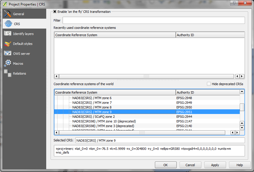 You must chosen the projection based on your study location; for more information on choosing an appropriate projection, see this Guide to Selecting Map Projections. Since our location was in Vancouver Island, we chose Universal Transverse Mercator (UTM), NAD83 (NSRS2007) /UTM zone 10N.
- Once you have chosen your Projection, click Next.
- This will bring you to the Define GRASS Region Window.
- Scroll to the country of your study area, and click Set.

- Then click Next.
- This will bring you to the Mapset Window.
- Name your new Mapset. We named ours Mapset.
- Click Next.
- Then click Finish.
 Your new mapset has now been created!
 - Now if you go back to the Plugins Tab, you can see that the tools are no longer grayed out. Depending on the computer you are using you may have to open the mapset every time you open and close QGIS.
- In order to do this, go to the Plugins Tab.
- Click GRASS
- Lastly, click Open Mapset.

Workspace Setup
Before beginning any data processing, the data must be added and the region must be set up.
Adding Vector Layers to QGIS
- To add vector layers, click the Add Vectors layer button at the top left of the screen.

- Browse to the location where you saved your data.
- Click Open.

- For this project we added the following vectors: Vancouver Island boundary, lakes, parks, landcover, grey wolf range (both polygon and points), hunting camps, and deforested areas.
- These layers will appear in the Table of Contents (TOC) on the left.
Adding Raster Layers to QGIS
- To add a raster layer, click the Add Raster Layer button.

- Navigate to the desired folder using the Browse button.
- Chose the w001001.adf file.
- Then click Open. These layers will show up in the TOC on the left. The raster layers we added to the project included: Road Density and the DEM.
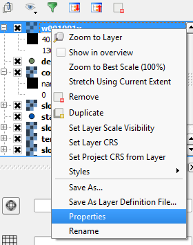
- In the TOC, right click on the layer that says w001001.
- Click on Properties.
- Within the Layer Properties, go to the General Tab.
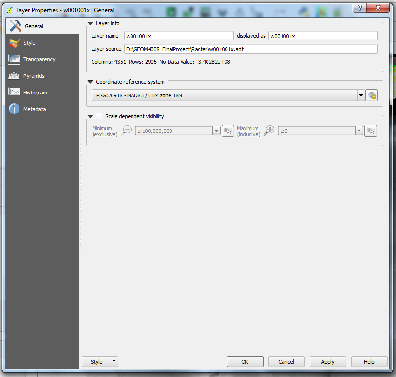
- Under Display Name, give the layer an appropriate name. For example, DEM.

- Next, go to the Style Tab.

- Change the Color Map option to be Pseudocolour.
- Then click OK.


Editing the Current GRASS Region
It is very important to edit the Current GRASS Region in order to specify the processing extents and resolution.
- To do this, go to the Plugins Tab.
- Click on GRASS.
- Then click the Edit Current GRASS Region Button.
- The extent can be created by drawing an area of interest around your boundary layer.
- Next the resolution must be changed. Change the cell width and cell height. We changed our cell width and height to be 50. This may be dependent on your data. Originally we tried a cell size of 90; however, this produced images that were too course. We also tried a a cell size of 10; however, this would not run.
- After you have changed the cell size click OK.
Data Processing
The data processing steps will set up all your layers in the proper formats to be used in the landscape permeability evaluation.
Clipping Vector Layers to AOI boundary
- To clip all the layers to your Area of Interest (AOI), go to the Vector Tab.
 Ex. we used the Vancouver Island boundary files as our AOI.
 - Click Geoprocessing Tools.
- Then click Clip.
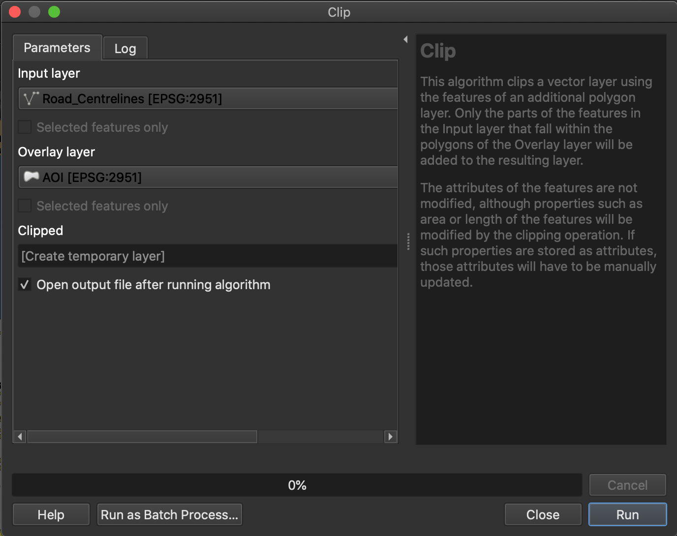
- The input vector layer is the layer that needs to be clipped.
 For example we had to clip our Roads file which originally contained all the Roads in BC.
 - The Clip layer is the layer you wish to be your AOI.

- Name the output shapefile and specify an appropriate location for it.
- Then Click OK.

Preforming a Union
A union must be completed on all of the vector layers that do not have full data coverage of the boundary file. The union will act to fill any NULL values in the dataset to be 0s instead; this will become important when using the Raster Calculator in later steps.
- To complete this process, go to the Vector Tab, click Geoprocessing Tools, and click Union.

- The input vector layer should be boundary file in all cases.
- The union layer should be any layer that does not have full coverage, as described above.
 We completed this process for lakes, parks, grey wolf range, landcover, deforested areas, and hunting camps.
 - Specify the location and name of the output shapefile. An example of how we named ours is Parks_U.
- Click OK.
- A geoprocessing box will pop up asking if you would like to add the new layer to the TOC.
- Click Yes.


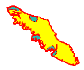
Figure 1: shows the Parks_U layer. The boundary area is shown in grey and the parks are shown in white.
Editing the Attribute Table
The attribute table must be edited on all the layers you preformed a union on. A CLASS field will house the unique values from which we will create our rasters later on.
- To open the attribute table, right click on the layer.
- Left click on Open Attribute Table.
- In order to edit, click the Editor Mode on.

- Create a new column by clicking New Column.

- The Add Column Window will pop up. Give the column a name. We named our CLASS.
- If you would like, you can give the column a comment; however, it is not necessary.
- Ensure the type is set to whole number (integer),
 with a width of 1.
- The click OK.
- In the new column CLASS, set the original boundary to be 1 and all the remaining attributes to be 2.
- The boundary can be distinguished by clicking on the numbers on the left side of the window. (seen in red).
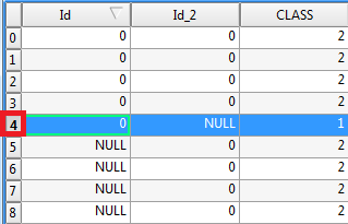
- As you click the numbers, sections of the map will become highlighted.
- Again, once you have found the boundary, put a 1 in the CLASS column and a 2 in the rest of the columns.
- To save changes click the Editor Mode button again.


Importing Vectors to GRASS Format
To use the GRASS Plugin all the layers must be imported into a GRASS format. For all the vector layers the tool v.in.ogr.qgis must be used.
- To do so go to the Plugins Tab.
- Click GRASS.
- Then click Open GRASS Tools.
- Next go to the Modules List Tab.
- In the Filter Box type v.in.ogr.qgis.
- Click on the Correct Tool.
- The tool will pop up.
- Use the drop down OGR vector layer arrow to select a layer to change to GRASS format.
- IMPORTANT NOTE: the layer must be on in the TOC for the drop down to function.
- Give the Output Vector Map a name.
 An example of our naming scheme is Deforest_U_G, where the "G" signifies that it is now in a GRASS vector format.
 - Click Run.

- Once the tool has successfully finished, click View Output.
 The layer will appear in the TOC.


Importing Rasters to GRASS Format
To use the GRASS Plugin, all the raster layers must also be imported into a GRASS format. For all the raster layers the tool r.in.gdal.qgis must be used.
- To do this, go to the Plugins Tab.
- Click GRASS.
- Then click Open GRASS Tools.
- Go to the Modules List Tab.
- In the Filter Box, type r.in.gdal.qgis.
- Click on the correct tool.
- The tool will popup.
- Use the drop down loaded layer arrow to select a layer to change to GRASS format.
- IMPORTANT NOTE: the layer must be on in the TOC and activated it show up in the dropdown menu.
- Give the Output Raster Map a name a click Run. An example of our naming scheme is DEM_G.
- Once the tool has successfully finished, click View Output. The layer will appear in the TOC.


Converting Vectors to Rasters
The convert vector to raster does exactly as the name sounds, converts GRASS vectors to GRASS rasters. All the vectors layers must be converted to raster in order to preform the reclassification in the following step. For our project we converted lakes, parks, landcover, grey wolf range, hunting camps, and deforestation.
- Go to the Plugins Tab.
- Click GRASS.
- Then click Open GRASS Tools.
- Go to the Modules List.
- In the Filter Box, type in v.to.rast.attr.
- Click on the correct tool.
 and the tool will then open.
 - Using the dropdown menu, select input vector layer you wish to rasterize.
- Remember, the layer must be on for it to appear in the dropdown menu.
- In the Attribute Field, select the CLASS layer that you created.
- Give the Output Raster Map a name.
- Click Run.
- Finally, click View Output.


Raster Data Processing: Creating the Slope Layer
To create a Slope layer, a Digital Elevation Model (DEM) must be given as the input.
- Go to the Plugins Tab.
- Click GRASS.
- Click Open GRASS Tools.
- Go to the Modules List.
- In the Filter Box, type Slope.

- Click the Slope Tool.

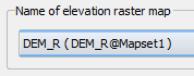
- Input the name of the Elevation Raster Map (DEM).
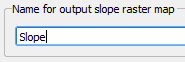
- Name the Output Slope Raster Map. Our output map was named Slope.
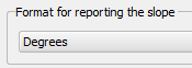
- The format for reporting the slope can be degrees or percent; we used degrees.
- Click Run.
- Lastly, click View Output.


Figure 2: Left: The DEM. Right: The resulting slope raster.
Reclassifying the Rasters According to Cost
In order to assign a cost value to each cell, we must perform a reclass on each raster. Before beginning the reclass, a textfile (.txt) must be written in which the reclass rules will be specified. This subjective process that should be based on scientific literature and expert opinion.
Creating the Reclass Rules Text Files
- For each unique pixel value in a raster, the reclass rules will dictate the assigned cost (i.e. the level of difficulty, from 1 to 10) that a wolf would have traveling across it. For example, any water pixel in the lakes raster, was assigned a cost of 7. The cost value of 7 was assigned because water poses a barrier to wolf movement; however, the wolves can swim if necessary.

- In the image shown above, the first column on the left indicates each unique pixel value in the raster (recall, for the layers in which a union was required,these values would be 1 (the boundary) and 2 (ex.lakes)). The second column indicates the cost value you wish to reassign to each pixel.
- If the raster has more than two unique values, then you can assign a single cost value to a range of slope values. This example is demonstrated below using our Slope Raster.

- For further help creating the reclass rule files see r.reclass GRASS Help
Running the Reclass Tool
Next you must actually run the reclass using the r.class tool.
- Go to the Plugins Tab.
- Click GRASS.
- Click Open GRASS Tools.
- Go to the Modules List.
- In the Filter Box, type in r.reclass.

- Click on the correct tool.

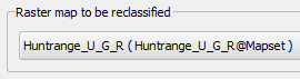
- Input the raster map to be reclassified.
- For the File Containing Reclass Rules parameter, Browse to the location of your saved reclass rules text file.
- Specify an Output Raster Map name. For example we called ours Huntrange_Reclass.
- Now click Run.
- Then, click View Output.


Combining the Cost Rasters in the Map Calculator
To create a cost raster that displays the cumulative cost of moving over the land, all the individual cost rasters must be added together using the Raster Map Calculator.
- Go to the Plugins Tab.
- Click GRASS.
- Click Open GRASS Tools.
- Go to the Modules List.
- In the Filter Box, type in r.mapcalculator.
- Click on the map calculator tool.
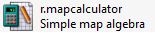

Figure 3: Unfortunately, the r.mapcalculator tool can only take in 6 input rasters. Since we had 8 cost factors, the calculation needed to be done in two steps, shown above.
- Click Run.
- Click View Output.

Figure 4: The final Master Cost Raster created by adding all the individual cost rasters together. The lighter areas indicate cells with high cost to movement (i.e. represent barriers or danger), and the darker areas show cells with lower cost.
Evaluating the Least Cost Paths and Least Cost Corridors
The Wolf Ranges
Before starting the actual evaluation, look at Figure 5 below. This shows the locations of the fictitious wolf ranges (i.e. areas where metapopulations of wolves are known to reside). The ranges are labeled A through D, from North to South, respectively. The goal of this analysis was to identify which paths pose the least resistant/danger to movement between each of these ranges.
 ::
::

Figure 5: The location of wolf ranges A, B, C, and D.
Evaluating Least Cost Path and Corridor between Wolf Ranges A and D
For this example, the least cost path and corridor from wolf ranges A to D were calculated. The first step in actually evaluating a cost path/corridor, is to calculate an accumulated cost surface from a starting point (A); this is done using r.walk. The second step is to run r.drain on the results from r.walk; in this step the destination (D) is specified. The output from this will be the least cost path from point A to D. This path should then be converted to a vector in order to create an editable line.
To generate the least cost corridors between ranges A and D, another accumulated cost surface must be created, this time, using point D as the starting point. The final step is to add these two accumulated cost surface rasters together, which will create the cost corridor.
Generating an Accumulated Cost Surface using r.walk
The r.walk.vect tool creates an accumulative cost distance value for each cell compared to the specified source location. This means that cells farther from the source feature will receive a higher cost distance value than cells closer to the source feature. This accumulated cost distance surface is a required input of the r.drain tool which actually generates the least cost path. In our example we wanted to inspect the path from wolf range A to D, so location A would be the starting point.
- Go to the Plugins Tab.
- Click GRASS.
- Click Open GRASS Tools.
- Go to the Modules List.
- In the filter box type in r.walk.
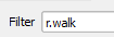
- Click on the r.walk.vect tool.

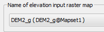
- In the Name of Elevation Input Raster Map parameter, select the DEM.
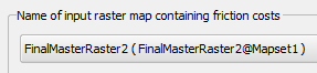
- In the Name of Input Raster Map Containing Friction Costs parameter, insert the master cost raster.
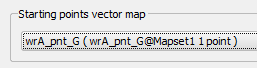
- In the Starting Points Vector Map parameter, select the starting location point. For our example, we wanted to start at Wolf Range A.
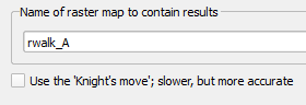
- Specify a output raster map name and deselect the option to Use the 'Knight's move'. For example we called ours rwalk_A.
- Now click Run.
- Then click View Output.
- Once your map has appeared, right click on the layer in the TOC.
- Left click on properties.
- Got to the Style Tab
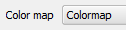
- In the Colormap box, use the dropdown menu and click colormap.
- Now go to the Colormap Tab.

- In the classification mode box, use the up arrows to make 8 classes.

- Click classify.


Figure 6: The accumulated cost surface raster for wolf range A .
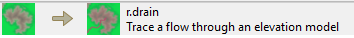
Generating Least Cost Paths using r.drain
r.drain creates the least cost path between the staring point and the destination. Although this tool was originally designed to be used in a hydrology context (hence the prompt for an elevation raster), it functions in the same manner for any accumulated cost surface raster.
- Go to the Plugins Tab.
- Click GRASS.
- Click Open GRASS Tools.
- Go to the Modules List.
- In the filter box type in r.drain.

- Click on the r.drain tool.
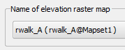
- In the Name of Elevation Raster Map box, use the dropdown menu to select rwalk_A.
- Give the output raster map a name. An example of our naming scheme would be r.drainAD.
- Next you must input the coordinates of the starting point. Contrary to it's decriptor, this point will actually be the destination point, in our case, this was wolf range D. Recall, the starting point (wolf range A) was previously specified in the r.walk tool to create the accumulated cost surface.
- The coordinates can be determined by using the Pan Map tool (in the upper left corner).

- Hold the Pan Map tool over the destination point The coordinates can be seen in the left hand corner.
- Write these coordinates down and then place them in the starting points box.
- The result is a path that goes from Wolf Habitat A to Wolf Habitat D. (See Figure 7)


Figure 7: The least cost path from wolf range A to D. It is hard to see since it is a raster. In the next step we will convert it to a vector and better symbolize it.
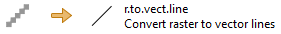
Converting the Least Cost Paths to Vectors
The r.to.vect.line tool can change the raster path created from r.drain from a raster to vector line. This is highly recommended since it will create a line who's appearance editable.
- Go to the Plugins Tab.
- Click GRASS.
- Click Open GRASS Tools.
- Go to the Modules List.
- In the filter box, type in r.to.vect.line.
- Click on the correct tool.
- The input raster map should be r.drainAD.
- The output vector line should be named something appropriate to what your path represents. We named ours adpath.
- Click Run.
- Then click View Output.


Preparing to Generate a Least Cost Corridor
To create a least cost corridor between to locations, two accumulated cost surfaces must be generated for the corresponding start and end locations. In this example, we already have the accumulated cost surface for wolf range A; now we need a second accumulated cost surface surface for wolf range D. This will be done by running the r.walk.vect again; however, this time point D is the starting point. The second step in creating the corridor is to add these two accumulated cost surfaces together, this part will be addresses in the following section.
- To create the second accumulated cost surface, refer to the "Generating an Accumulated Cost Surface using r.walk" section above.
- Be sure to change the starting point to be the appropriate layer for your specific analysis. In this case, the new input for us was wolf range D (wrD_pnt_G).
- Don't forget to rename your output appropriately as well. We named ours rwalk_D.
- The resulting r.walk map for wolf range D is shown below.


Figure 8: The accumulated cost surface raster for wolf range D .
Generating a Least Cost Corridor between Two Locations
The final step to create a least cost corridor between two locations is to add the respective accumulated cost surfaces together using the r.mapcalc tool. This tool is a graphical version of the r.mapcalulator tool and was chosen this time just to give you experience working with both interfaces.
- Go to the Plugins Tab.
- Click on GRASS.
- Click Open GRASS Tools.
- Go to the Modules List.
- In the filter box, type in r.mapclac.
- Click on the r.mapcalc tool.
- In the window, create the addition equation that adds the two accumulated cost surfaces together. For example, our equation added rwalk_A and rwalk_D.
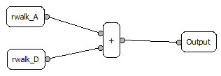
- In the output, name the map something appropriate. We chose adcorridor.
- Click Run.
- Finally, click View Output.


Figure 9: The least cost path from wolf range A to D overlaid on the corresponding least cost corridor map.
Conclusion
Repeating the r.walk and r.drain processes of creating least cost paths and corridors for each combination of starting and ending destinations (AB,AC,AD,BC,BD,CD). You can create a map that resembles Figure 10 by turning on all these created layers in the TOC. This map shows all the possible least cost paths to each wolf range overlaid on an cumulative least cost corridor. This cumulative least cost corridor was created by adding all of the accumulated cost surfaces for each starting point together, as shown in Figure 11. Sometimes, it might be appropriate to overlay the paths on other surfaces, such as the master cost raster (e.g. Figure 12). This map just emphasizes that the paths in actual fact do follow the least costly (lighter cells) routes. For example, the large whiter circles represent the radius around the hunt camps, which were assigned a cost factor of 9; as a result, the paths serve around all of these dangerous areas.

Figure 10: (Above) The final map showing all the possible least cost paths to each wolf range overlaid on a cumulative least cost corridor raster .

Figure 11: (Above) The r.mapcalc graphical equation used to add all of the accumulated cost surfaces to create the cumulative least cost corridor raster seen in figure 10.

Figure 12: (Above) All the possible least cost paths overlaid on the master cost raster. This emphasizes that most of the high cost areas (shown in lighter tones) are being avoided by the paths.
![]()
Helpful Links
Welcome to the Quantum GIS Project