Difference between revisions of "Exploring Hydrological Analyses using SAGA GIS"
Siefatfatin (talk | contribs) |
|||
| (38 intermediate revisions by 4 users not shown) | |||
| Line 92: | Line 92: | ||
'' Figure 2. Digital Elevation Model for Lake Okanagan, British Columbia, Canada (Source: NRCan, 2013) '' |
'' Figure 2. Digital Elevation Model for Lake Okanagan, British Columbia, Canada (Source: NRCan, 2013) '' |
||
[[Image:terrainanalysis.png|250px]] |
|||
===Saving Data in SAGA GIS=== |
===Saving Data in SAGA GIS=== |
||
In order for a user to save imported data or data that is generated through the use of an analysis tool, they must save each raster file individually. This is because the files do not save automatically anywhere on the computer and saving all your work as one SAGA project (.sprj) does not not actually save the individual raster files; and if the files are not saved they cannot be re-manipulated of processed if the document is closed or crashes. To save raster files properly in SAGA GIS: |
In order for a user to save imported data or data that is generated through the use of an analysis tool, they must save each raster file individually. This is because the files do not save automatically anywhere on the computer and saving all your work as one SAGA project (.sprj) does not not actually save the individual raster files; and if the files are not saved they cannot be re-manipulated of processed if the document is closed or crashes. To save raster files properly in SAGA GIS: |
||
[[Image: |
[[Image:savingdataas.png|250px]] |
||
* Navigate to the raster file from the files list in the '''Data''' tab of the ''workspace''. |
* Navigate to the raster file from the files list in the '''Data''' tab of the ''workspace''. |
||
| Line 113: | Line 111: | ||
* Navigate to the toolset titled '''Projection - Proj.4''' and expand it by clicking the small plus sign button. |
* Navigate to the toolset titled '''Projection - Proj.4''' and expand it by clicking the small plus sign button. |
||
[[Image: |
[[Image:1Proj4command_line.png|250px]] |
||
* Now go down to the tool titled '''Proj.4(Command Line Arguments,Grid)'''. |
* Now go down to the tool titled '''Proj.4 (Command Line Arguments,Grid)'''. |
||
* You will now see a dialogue box pop-up with two major fields, the first called Source Parameters and the second called Target Parameters. |
* You will now see a dialogue box pop-up with two major fields, the first called Source Parameters and the second called Target Parameters. |
||
* In the second row of Source Parameters, called Grid System, you will need to use the drop down menu to select the grid system under which your elevation dataset is listed (based on what is written in the data section of the workspace window. |
* In the second row of Source Parameters, called Grid System, you will need to use the drop down menu to select the grid system under which your elevation dataset is listed (based on what is written in the data section of the workspace window. |
||
[[Image: |
[[Image:2source_parameters.png|250px]] |
||
* Next, you need to select your DEM file using the drop down menu of the row titled '''source'''. |
* Next, you need to select your DEM file using the drop down menu of the row titled '''source'''. |
||
| Line 132: | Line 130: | ||
* Please make sure that the appropriate cellsize is defined, otherwise your newly projected DEM file won't work properly for the hydrological analysis. Your cellsize input needs to be the same as the cellsize on the original DEM. ''For the this tutorial on ''Lake Okanagan'' watershed delineation, the cellsize was set to 30.'' |
* Please make sure that the appropriate cellsize is defined, otherwise your newly projected DEM file won't work properly for the hydrological analysis. Your cellsize input needs to be the same as the cellsize on the original DEM. ''For the this tutorial on ''Lake Okanagan'' watershed delineation, the cellsize was set to 30.'' |
||
[[Image: |
[[Image:3cell_size.png|250px]] |
||
* After this the only thing left to do is to click '''Okay'''. |
* After this the only thing left to do is to click '''Okay'''. |
||
| Line 156: | Line 154: | ||
* Once the Pre-processing menu has opened up beside the Terrain Analysis, you will need to locate the fill sinks tool titled '''Fill Sinks (Wang Lui)'''. |
* Once the Pre-processing menu has opened up beside the Terrain Analysis, you will need to locate the fill sinks tool titled '''Fill Sinks (Wang Lui)'''. |
||
[[Image: |
[[Image:1_sinking.png|250px]] |
||
* Once you have opened the '''Fill Sinks (Wang Lui)''' tab, you select your grid system (under which your DEM data is saved) through the drop down menu beside the row entitled '''Grid System'''. |
* Once you have opened the '''Fill Sinks (Wang Lui)''' tab, you select your grid system (under which your DEM data is saved) through the drop down menu beside the row entitled '''Grid System'''. |
||
| Line 162: | Line 160: | ||
* Once you have done this, make sure the fields '''Filled DEM''','''Flow Directions''', and '''Watershed Basins''' through their drop down menus have '''[create]''' selected. |
* Once you have done this, make sure the fields '''Filled DEM''','''Flow Directions''', and '''Watershed Basins''' through their drop down menus have '''[create]''' selected. |
||
[[Image: |
[[Image:2_wanglui.png|250px]] |
||
* The next step is to click '''Okay''', since you generally don't need to edit the optional Minimum Slope row. |
* The next step is to click '''Okay''', since you generally don't need to edit the optional Minimum Slope row. |
||
| Line 179: | Line 177: | ||
* Once there expand the toolset using the small plus sign button beside the toolset name. |
* Once there expand the toolset using the small plus sign button beside the toolset name. |
||
* Double click '''Slope, Aspect, Curvature''', and this will open a window for the analysis tool dialogue box. |
* Double click '''Slope, Aspect, Curvature''', and this will open a window for the analysis tool dialogue box. |
||
* Select your grid system, under which your DEM data file is located, with the drop down menu on the right of the window in the row |
* Select your grid system, under which your DEM data file is located, with the drop down menu on the right of the window in the row labeled '''Grid System'''. |
||
* You then go down to the row '''Elevation''' and go to the right and select your elevation data, which is your DEM file, through the drop down menu. |
* You then go down to the row '''Elevation''' and go to the right and select your elevation data, which is your DEM file, through the drop down menu. |
||
* To create your Slope and Aspect maps ensure that you select '''[create]''' on the right drop down menu for those respective rows. |
* To create your Slope and Aspect maps ensure that you select '''[create]''' on the right drop down menu for those respective rows. |
||
| Line 197: | Line 195: | ||
'' Figure 5. Slope map of the Lake Okanagan, British Columbia, Canada study region. '' |
'' Figure 5. Slope map of the Lake Okanagan, British Columbia, Canada study region. '' |
||
===Converting a Vector Polygon to Raster=== |
|||
'''EDIT THE WATERSHED PORTION ONLY (ALL OF IT) EVERYTHING ELSE IS GOOD.''' |
|||
This section of the tutorial will run through the procedures that are required to take a file that is in vector polygon format and convert it into raster format. This step is very important since it is required for one of the inputs for the next part of the hydrological analysis, where we evaluate watershed delineation. When creating a watershed it is required that a target area be specified based on which the watershed will be built, and this area needs to be a hydrologic feature like a Lake or River. Due to the fact that hydrologic features are generally not found in raster format it is important to follow the procedures of this section to convert the polygon into raster for a more accurate SAGA GIS analysis. |
|||
To convert vector to raster: |
|||
* First navigate to the '''Modules''' tab of the main menu toolbar. |
|||
* Open the Modules tab by clicking on it and then navigate down the drop down list to '''Grid'''. |
|||
* In the Grid menu that should have opened after you navigated to the ''Grid'' selection, you will need to find the '''Gridding''' toolset. |
|||
* In this toolset go down the list to the '''Shapes to Grid''' tool and open it. |
|||
[[Image:ShapestoGrid.png]] |
|||
* The tool dialogue box will now open with many input options. |
|||
* The first two rows of the tool are labelled '''Shapes''' and '''Attribute''' and these options give the user the fields in which the vector polygon file that needs to be converted must be specified. So in the first row you will need to use the drop down menu and select the vector polygon file that needs to be converted. For this project the Okanagan Lake vector polygon was selected. |
|||
* In the second row you will need to select the attribute of the vector file that will determine the file outline boundaries. ''Note: because the file is just being converted in this case for the watershed delineation the any attribute can be chosen, and in this project the Object ID field was employed''. |
|||
* The next row titled '''Method for Multiple Values''' you will need to select the '''Mean''' option from the drop down menu. ''This tells the conversion algorithm to take the average if two or more alike values are found in the vector file''. |
|||
* The field called '''Method for Lines''' can be specified however you want. It just means that the outline of your vector polygon will either be thick or thin. ''For this project the thin option was employed''. |
|||
* '''Preferred Target Grid Type''' field will vary depending on the type of vector data file you have. In this project the vector polygon for Okanagan Lake was a 8 byte vector and so the '''Floating Point (8 byte)''' option was chosen. |
|||
* The last field '''Target Grid''' needs to be set to '''Grid''' so that SAGA knows that a new grid needs to be created. |
|||
* The Shapes to Grid tool can be seen below to help you better understand the procedures. |
|||
[[Image:ShapestoGridTool.png]] |
|||
* Once you have input all the required parameters for the tool click '''Okay''' and your vector polygon hydrologic feature will become a raster. Below the Okanagan lake raster is shown after being converted from a vector polygon. |
|||
[[Image:OkanaganLake.png]] |
|||
===Creating a Watershed map=== |
===Creating a Watershed map=== |
||
This section will run through the actual hydrological analysis of generating |
This section will run through the actual hydrological analysis of generating watershed maps for a region. In this specific tutorial the ''Okanagan Lake'' watershed is generated only, but the procedures would apply to any study region. To make a watershed map: |
||
* |
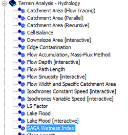
* Go to the workspace window's '''Modules''' Tab and scroll down to '''Terrain Analysis - Hydrology''' and expand it. |
||
* Scroll down to '''Upslope Area''' and open |
* Scroll down to '''Upslope Area''' and open the tool by double clicking. |
||
[[Image:1upslopearea.png|250px]] |
[[Image:1upslopearea.png|250px]] |
||
* Select your grid system through the drop down menu on the right side of the window on the '''Grid System''' row . |
* Select your grid system through the drop down menu on the right side of the window on the '''Grid System''' row . |
||
* Go down to the row titled '''Target Area''' and select your area of interest |
* Go down to the row titled '''Target Area''' and select your area of interest, which is the converted vector hydrologic feature on which the watershed will be based. In this tutorial the Target Area is the ''Okanagan Lake boundary'' raster file. |
||
* Go down to the '''Elevation''' row and select your DEM data from the drop down menu on the right side of the window. |
* Go down to the '''Elevation''' row and select your '''Filled DEM''' data from the drop down menu on the right side of the window. |
||
* Ensure that the row titled '''Sink Routes''' has '''[not set]''' selected through the drop down menu |
* Ensure that the row titled '''Sink Routes''' has '''[not set]''' selected through the drop down menu. This field is specified as [not set] because the filled DEM already accounts for the sink routes of the data. |
||
* Go down to the row titled '''Upslope Area''' and make sure '''[create]''' is selected in the drop down menu. |
* Go down to the row titled '''Upslope Area''' and make sure '''[create]''' is selected in the drop down menu. This is the field that tells the algorithm to output the the watershed map which is also known as an upslope area map. |
||
* Go under '''Options''' and to the row '''Method''' and make sure '''Deterministic 8''' is selected from the drop down menu. |
* Go under '''Options''' and to the row titled '''Method''' and make sure '''Deterministic 8''' is selected from the drop down menu. ''Note: The Deterministic 8 (D8) algorithm is chosen in this project because it is found to be the best option when generating watershed maps. This D8 algorithm assumes that each cell of the Filled DEM has unidirectional water flow, whereas the other algorithms assume that one cell can have water flowing in multiple directions. To make a more accurate and understandable watershed delineation map the D8 algorithm is best''. |
||
* Now the next field is titled '''Convergence''' and for this row it is advised that you '''please ignore''' the field and leave the default value. It is important to leave the field untouched because this convergence factor only applies it you are using the ''multiple flow direction'' algorithm but because we have use the D8 algorithm this field will not apply to the output. |
|||
[[Image:2upslopearea.png|250px]] |
[[Image:2upslopearea.png|250px]] |
||
| ⚫ | |||
| ⚫ | |||
* This creates your Watershed Map. |
* This creates your Watershed Map. |
||
[[Image:UpslopeArea.png|400px]] |
[[Image:UpslopeArea.png|400px]] |
||
'' Figure 6. Watershed of Lake Okanagan, British Columbia, Canada. '' |
'' Figure 6. Watershed of Lake Okanagan, British Columbia, Canada. '' |
||
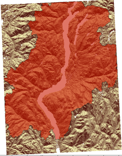
Now as seen in Figure 6 an excellent watershed delineation map has been generated for the study region, however you can also see that the watershed map is projected onto just a white background causing the information to be ambiguous and provide no geospatial meaning. In order for hydrologists and/or researchers in the real world to use this map successfully you would definitely need to drape this map over an other map (like a DEM, Basemap of the study region or aspect map) that provides geospatial context to the information so that researchers can actually see which areas of the study region contribute water flow into Okanagan Lake. In this project the watershed was given geospatial context by draping it over the aspect map because this map clearly depicts the landscape of the study region and help pinpoint areas that contribute water flow to the target area. |
|||
[[Image:UpslopeAreaWithAspect.png|400px]] |
[[Image:UpslopeAreaWithAspect.png|400px]] |
||
'' Figure 7. Watershed of Lake Okanagan, British Columbia, Canada shown draped over the aspect map in order to make the data more meaningful. '' |
'' Figure 7. Watershed of Lake Okanagan, British Columbia, Canada shown draped over the aspect map in order to make the data more meaningful. '' |
||
In Figure 7 you can see the watershed map draped over the aspect map. To drape the watershed over other maps you first need to convert the raster watershed file into a vector polygon and to do this: |
|||
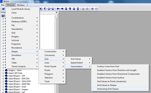
* You will first need to open the tool called '''Vectorising Grid Classes''' by navigating through the menus of the main toolbar using the following steps: '''Modules | Shapes | Grid | Vectorization | Vectorising Grid Classes'''. |
|||
[[Image:stepsforvectorising.png|300px]] |
|||
* Once the tool's dialogue box has opened you will need to once again select your '''grid system''' from the drop down list of the respective row. |
|||
* Next go down to the '''Grid''' field and input the '''Upslope Area''' map that was created for the watershed map. |
|||
* In the field titled '''Polygons''' may sure that the selection column is set as '''[create]''' so that the algorithm knows that a vector polygon needs to be generated. |
|||
* The next field called '''Class selection should be set as '''All Classes''' and the '''class identifier''' should be set as '''1'''. This field will specify how many classes you want generated in the output vector polygon. |
|||
* The last input field called '''Vectorised class as...''' should be set to '''one single (multi-)polygon object''' because we want only one single polygon created. ''The other option of this field would create a vector file of the upslope area but with lots of polygons to build it, and using the one single option you will get one polygon which want is needed to drape it over the aspect map''. |
|||
* Now click '''Okay''' and a new vector file will be generated of the watershed map. |
|||
[[Image:ToolforVectorisation.png|500px]] |
|||
The above steps describe the steps required to convert a raster to vector polygon so that the watershed map can be draped over the aspect map. Once the watershed map has been vectorised further steps can be taken to drape it over other maps for geospatial context. To do this: |
|||
* Go to the '''Data''' tab of the workspace window and find the '''upslope area vector polygon''' file. |
|||
* Click on the name of the file to select it and when it is highlighted go to the '''properties window''' which located on the right hand side of the screen. |
|||
* In the properties window ensure that you are in the '''Settings''' and then navigate to up to the field titled '''Transparency [%]'''. |
|||
* In this field you can input any value you prefer based on how transparent you would like your watershed map to look when it is displayed over the aspect map. For the Okanagan Lake study area a transparency of '''40''' of selected. |
|||
* Once the transparency percentage has been specified click '''Apply''' and then '''Save''' at the bottom of the properties window. |
|||
* Now go back to the '''Data''' tab of the workspace window and right click on the watershed vector file. |
|||
* Select the '''Add layer to Map''' option. |
|||
* In the '''Map Selection Window that pops up select the '''Upslope area''' map. |
|||
* Finally click '''OK''' and now your Watershed map is fully completed and has great geospatial information along with its hydrological information just like Figure 7. |
|||
===Creating a Wetness Index Map=== |
===Creating a Wetness Index Map=== |
||
This section will run through the analysis of defining a region's wetness, which describes how susceptible specific areas in a study region are to becoming saturated if high inputs of precipitation occur in a relatively short amount of time. To run a wetness index analysis conduct the following: |
This section will run through the analysis of defining a region's wetness, which describes how susceptible specific areas in a study region are to becoming saturated if high inputs of precipitation occur in a relatively short amount of time. To run a wetness index analysis conduct the following: |
||
* In the workspace window under |
* In the workspace window under the '''Modules'' tab scroll down to '''Terrain Analysis - Hydrology''' and expand it using the small plus sign button. |
||
* Scroll down to '''SAGA Wetness Index''' tool and double click it to open the dialogue box to the analysis tool. |
* Scroll down to '''SAGA Wetness Index''' tool and double click it to open the dialogue box to the analysis tool dialogue box. |
||
[[Image:1creatingwatershed.png|250px]] |
[[Image:1creatingwatershed.png|250px]] |
||
| Line 245: | Line 286: | ||
'' Figure 8. Map displaying the Wetness Index of the Lake Okanagan Region; where red shows highest wetness and blue shows driest areas. '' |
'' Figure 8. Map displaying the Wetness Index of the Lake Okanagan Region; where red shows highest wetness and blue shows driest areas. '' |
||
==Conclusion== |
|||
== Conclusion -- Completed Objectives == |
|||
Better understand how the software works. <br> |
|||
Steps need to be taken in order to achieve the desired output maps that are both accurate based on the input data and informative for the specific study region and hydrologic information. |
|||
==References== |
==References== |
||
Latest revision as of 18:01, 27 December 2013
Contents
- 1 Purpose of Tutorial
- 2 Introduction to SAGA GIS
- 3 Hydrology Definitions
- 4 Introduction to Project Tutorial
- 5 Data
- 6 Methods Conducted in SAGA GIS for Hydrological Analysis
- 6.1 SAGA GIS Basic Setup
- 6.2 Opening SAGA GIS
- 6.3 Importing DEM
- 6.4 Saving Data in SAGA GIS
- 6.5 Projecting the Data Properly to Conduct Analysis
- 6.6 Filling in the Sinks of a DEM
- 6.7 Aspect Maps and Slope Maps
- 6.8 Converting a Vector Polygon to Raster
- 6.9 Creating a Watershed map
- 6.10 Creating a Wetness Index Map
- 7 Conclusion -- Completed Objectives
- 8 References
Purpose of Tutorial
This Wiki has been produced for the GEOM 4008 - Advanced Topics in Geographic Information Systems class at Carleton University for the purposes of exploring and describing the methods of Hydrological Analyses using FOSS4G, in specific SAGA GIS. The main objective for this wiki tutorial is to help future users of SAGA GIS's hydrological toolset better understand how the software works and exactly what steps need to be taken in order to achieve the desired output maps that are both accurate based on the input data and informative for the specific study region and hydrologic information.
Introduction to SAGA GIS
SAGA GIS stands for System for Automated Geoscienific Analyses. It is a Geographic Information System software program designed to easily and effectively implement spatial algorithms, for real world situations and education. This geospatial software offers a continuously growing comprehensive set of geoscientific tools/methods. The program has an accessible graphical user interface with various visualization options to help users easily operate the various analysis tools. SAGA is capable of running on both Windows and Linux operating systems. SAGA GIS also comes at no cost for the user because it is a Free Open Source Software for Geospatial analysis (FOSS4G). Being a FOSS4G program allows a high degree of freedom for the user; it allows the user to run the program for any geoscientific purpose, to modify the program, to redistribute copies of it, and to improve the program while sharing those improvements with the general public. More information about this program is available at SAGA GIS's Website.
Hydrology Definitions
- Hydrology: Hydrology is the study of the movement, and distribution of water in all parts of the Hydrosphere. The focus of this project is on Watershed Hydrology which deals with surface runoff within specific watersheds, based on regional topography (USGS, 2013).
- Watershed: A watershed (also known as catchment area or drainage basin) is the area of land where surface water converges to the same lower elevation base point. In this projectLake Okanagan is the baseline of the basin for all the surface runoff (USGS, 2013).
- Topographic Wetness Index (TWI): The topographic wetness index is a method used to monitor rainfall and runoff. The analysis describes the aptness of an area to be saturated based on the surrounding area's slope characteristics and porosity of the ground surface (Olaya & Conrad, 2009).
Introduction to Project Tutorial
This project will focus on hydrological analysis of Okanagan Lake which is part of a popular tourist region located in south central British Columbia, Canada. There will be a focus on Aspect mapping,Slope mapping,Watershed Delineation mapping and Wetness Index mapping, through the use of SAGA GIS and its built in terrain analysis - hydrology module tools. This project aims to determine areas of the Okanagan region that contribute water to Okanagan Lake, and also what areas are susceptible to flooding during high precipitation events based on the slope characteristics and soil properties of specific land surfaces in the study region. By the end of this tutorial new users to SAGA software should be able to fully and efficiently conduct watershed and wetness index analyses using a raster DEM of any region in the world.
Data
In order to conduct this tutorial and appropriately follow the procedures you will first need to download data that is hydrologically correct and has elevation values for the entire study region. For the hydrological analyses you will essentially need to download a fully processed digital elevation model (DEM) for the region you are interested in. One important thing to note when retrieving DEMs is to make sure that if the elevation data for your area of interest is in separate tiles and requires that they be merged, you must insure that the DEMs were developed at the same resolution, cell size and during the same project. If these ideas are not followed it is possible that the tiles have cliffs within the DEM where the merging has occurred. In specific to this tutorial the study area will be the Lake Okanaganregion for which a processed DEM has been acquired from the Natural Resources Canada Geospatial Data Extraction Tool. This data extraction website is great for getting good processed elevation data for much of Canada and also contains other data files for many projects.
| Data | Data Format | Data Source |
|---|---|---|
| Okanagan Lake | Vector Polygon | Geogratis Layer: Hydrography / Producer: Natural Resources Canada |
| Digital Elevation Model (DEM) | Raster | Geogratis Layer: Canadian Digital Elevation Model Data / Producer: Natural Resources Canada |
| Okanagan Region Aspect Map | Raster | Created Data |
| Okanagan Region Slope Map | Raster | Created Data |
| DEM with Filled Sinks | Raster | Created Data |
| Okanagan Lake Boundary | Raster | Created Data |
| Catchment Area | Raster | Created Data |
| Topographic Wetness | Raster | Created Data |
Methods Conducted in SAGA GIS for Hydrological Analysis
SAGA GIS Basic Setup
Before you start setting up SAGA GIS for use it is recommended that you acquire the data which you plan to use for your project; be aware of where your data is located in a folder and make sure all of the data you are using is located in that folder.
Opening SAGA GIS
To run your hydrological analyses ensure that SAGA GIS is properly installed onto your computer and functional. If you do not have SAGA GIS you can download it at SAGA GIS homepage.
- If installed and functional, one simply has to locate and click the SAGA GIS icon
this will open the initial SAGA GIS window.
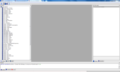
- Once SAGA GIS has been opened your user interface will be shown as below.
Figure 1. Screenshot of what the SAGA GIS graphical user interface looks like at start up
Importing DEM
This section will instruct you how to appropriately bring in a processed DEM into SAGA GIS so that you can effectively conduct a hydrological analysis.
- In the SAGA GIS graphical user interface (gui) you will first need to navigate to the Modules pull down menu located within the main menu toolbar at the top of the screen.

- In the Modules menu navigate to File and then to GDAL/OGR and open the GDAL: Import Raster command.
- Once the Import Raster dialogue box has opened you will see that the first row has the word File in the left column and nothing in the right column. You need to click on the empty column, which will result in the box displaying an ellipsis (...) button. You will then click on this button, which will open a file browser, and navigate to your DEM file. When you have located your elevation model file click Open and then in the Import Raster dialogue box click Okay. Note: When downloading when importing a DEM into SAGA, it can be in any raster format (e.g. .rst, .GRID, .tiff) but the tiff format is preferred.
- After you have started the importation process for the DEM file, you can see the progress of the module in the messages window located at the bottom portion of the SAGA gui. When the message window displays Module Execution Succeeded, your DEM has been correctly imported into SAGA.
- One aspect that is important to remember when importing any file into SAGA including the DEM raster file, is that the imported file will show up in the data tab of the workspace,
 however in order to visually see your data you need to double click on the file name which will open a new window entitled Add layer to selected map, then select new and click OK.
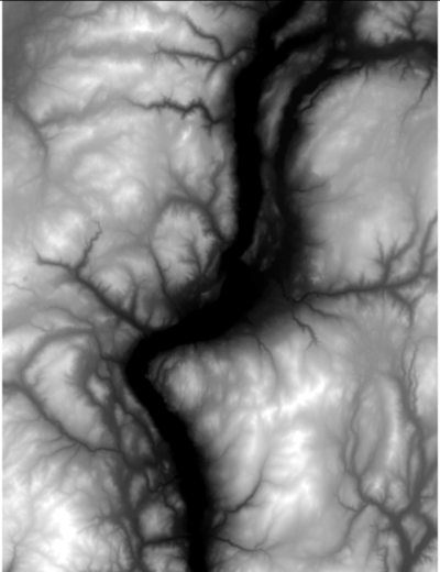
 - Now the DEM is been completely and accurately imported into SAGA GIS and will be displayed like Figure 2.
Figure 2. Digital Elevation Model for Lake Okanagan, British Columbia, Canada (Source: NRCan, 2013)
Saving Data in SAGA GIS
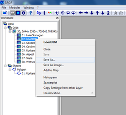
In order for a user to save imported data or data that is generated through the use of an analysis tool, they must save each raster file individually. This is because the files do not save automatically anywhere on the computer and saving all your work as one SAGA project (.sprj) does not not actually save the individual raster files; and if the files are not saved they cannot be re-manipulated of processed if the document is closed or crashes. To save raster files properly in SAGA GIS:
- Navigate to the raster file from the files list in the Data tab of the workspace.
- Now right click the file name and scroll down to Save As....
- Clicking save as will open a new window that allows you to specific where you want the file to be saved, what you want to name it and what format it should be in (Note: the .sgrd extension is the native grid format for SAGA GIS and generally works best).
- Once all the information has been specified in this Save Grid window, click Save. Your raster data has now been successfully saved.
Projecting the Data Properly to Conduct Analysis
In SAGA GIS you will have to begin your analyses by first projecting your DEM file into a Universal Transverse Mercator (UTM) projection system because SAGA works best of this coordinate reference system in regard to hydrology tools. If your DEM was already in a UTM system and in the correct zone for the study region, you can skip this step, otherwise you need to go through the following steps to convert the original projection of the DEM file into a UTM zone system that SAGA can work in.
Steps for Projecting files in SAGA GIS:
- Look up your specific proj.4 code online for your area of interest at spatialreference.org. Note: Make sure that you find a code for your DEM that is in NAD83(CSRS) UTM and also ensure that you are projecting it into the correct UTM zone for your study region.
- Once you have the proj.4 code, you back into SAGA GIS, and open the Modules tab in the workspace window.
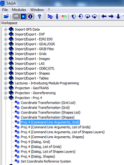
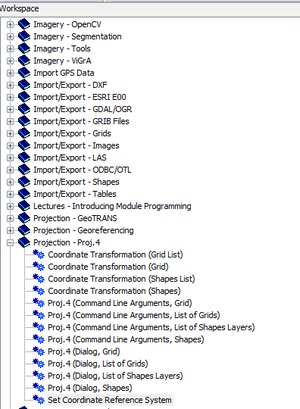
- Navigate to the toolset titled Projection - Proj.4 and expand it by clicking the small plus sign button.
- Now go down to the tool titled Proj.4 (Command Line Arguments,Grid).
- You will now see a dialogue box pop-up with two major fields, the first called Source Parameters and the second called Target Parameters.
- In the second row of Source Parameters, called Grid System, you will need to use the drop down menu to select the grid system under which your elevation dataset is listed (based on what is written in the data section of the workspace window.
- Next, you need to select your DEM file using the drop down menu of the row titled source.
- Inputting the DEM file into the dialogue box will automatically change the input of the first row called Source Projection Parameters to the appropriate projection.
- Now in the Target Parameters, type in the Proj.4 projection code retrieved from the spatial reference website.
- Leave the Create X/Y Grids box unchecked and proceed to the next row.
- In the Interpolation file select any surface interpolation you prefer from the drop down list (Natural Neighbor is used for this tutorial and it is generally a good idea depending on your project).
- In the last field of the dialogue box use the drop down menu once again and select user defined.
- The next step in the projection process is to click Okay.
- This will once again pop-up a new window that allows you to manipulate the user defined grid for your projection.
- In this user window the first four rows will already have correct inputs based on your Target Parameters, but you will need to input a defined parameters into the cellsize field.
- Please make sure that the appropriate cellsize is defined, otherwise your newly projected DEM file won't work properly for the hydrological analysis. Your cellsize input needs to be the same as the cellsize on the original DEM. For the this tutorial on Lake Okanagan watershed delineation, the cellsize was set to 30.
- After this the only thing left to do is to click Okay.
- You have now successfully re-projected the original DEM into proper UTM coordinates for your hydrological analysis.
- This projection tool provides the file with an internal coordinate reference system (CRS), however to apply a CRS to the actual raster file you need to use the Set Coordinate Reference System.
- The Set Coordinate Reference System tool is located under Module | Projections | Set Coordinate Reference System.
- In the tool window you will need to input the EPSG code for the projection that was applied to the DEM using the Proj.4 projection tool. This EPSG code can also be found at the spatial reference website.
- Once the EPSG code has been defined the Proj4 Parameters field will change automatically based on the projection code.
- Next, go down to the Grids field under the Data Objects section and click the empty column to display the browse button
 .
. - Clicking the browse button will take you to an internal pop-up window in which you will need to select your DEM file that you projected already and transfer it over to the right column which should be empty.
- Click Okay.
- Click Okay on the main dialogue box of the Set Coordinate Reference System tool as well.
- Finally your projection application of your DEM is complete and your raster file is ready for hydrological analyses.
Filling in the Sinks of a DEM
It is absolutely vital for people conducting hydrological analyses to fill in the sinks contained within digital elevation models. By filling in the these sink features you are essentially limiting the number of geometric artefacts, errors from specular reflection of water, and other errors in the elevation model caused by a variety of aspects. To fill in the sinks go through the following steps:
- Go to the Modules menu in the main toolbar.
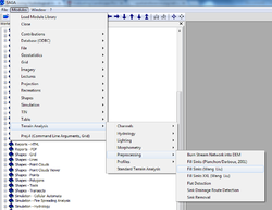
- Next navigate to the Terrain Analysis menu, expand it and then hover the mouse over Pre-processing.
- Once the Pre-processing menu has opened up beside the Terrain Analysis, you will need to locate the fill sinks tool titled Fill Sinks (Wang Lui).
- Once you have opened the Fill Sinks (Wang Lui) tab, you select your grid system (under which your DEM data is saved) through the drop down menu beside the row entitled Grid System.
- After selecting your grid system, you go to the row entitled DEM and select your DEM file through the drop down menu.
- Once you have done this, make sure the fields Filled DEM,Flow Directions, and Watershed Basins through their drop down menus have [create] selected.
- The next step is to click Okay, since you generally don't need to edit the optional Minimum Slope row.
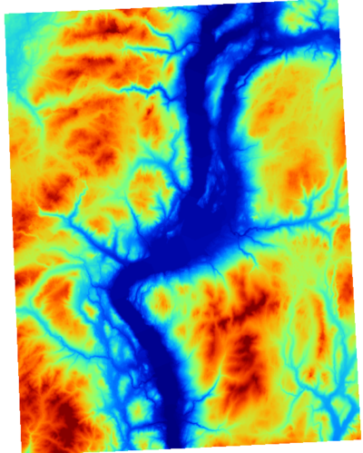
- After all of these steps you will have a new DEM file in which all the sinks are filled, thereby making your DEM a hydrologically correct one; and this is shown in Figure 3 for the Lake Okanagan DEM.
Figure 3. Digital Elevation Model for Lake Okanagan, British Columbia, Canada after all sinks had been filled in (Projection: NAD83(CSRS) UTM Zone 10N).
Aspect Maps and Slope Maps
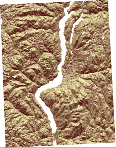
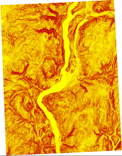
Aspect and slopes maps were created in this project tutorial because these maps are a great way to visualize the DEM information and allow you see what the topography looks like in the area as if you were flying over the region in an aircraft. To conduct these analyses go through the following procedures:
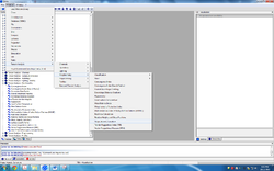
- Go to the workspace window of the SAGA GIS GUI and scroll down to the toolset titled Terrain Analysis - Morphometry
- Once there expand the toolset using the small plus sign button beside the toolset name.
- Double click Slope, Aspect, Curvature, and this will open a window for the analysis tool dialogue box.
- Select your grid system, under which your DEM data file is located, with the drop down menu on the right of the window in the row labeled Grid System.
- You then go down to the row Elevation and go to the right and select your elevation data, which is your DEM file, through the drop down menu.
- To create your Slope and Aspect maps ensure that you select [create] on the right drop down menu for those respective rows.
- Make sure that the rows titled Curvature, Plan Curvature, and Profile Curvature have [not set] selected in their respective drop down menus.
- In the row entitled Method you can choose whichever algorithm you desire, however it was found that the Fit 2.Degree Polynom (Zevenbergen & Thorne 1987) seems to work really well and so that is the one employed for the Okanagan Lake region.
- After completing these steps click Okay at the top right of the window.
- This will create your maps.
Figure 4. Aspect map of the Lake Okanagan study area.
Figure 5. Slope map of the Lake Okanagan, British Columbia, Canada study region.
Converting a Vector Polygon to Raster
This section of the tutorial will run through the procedures that are required to take a file that is in vector polygon format and convert it into raster format. This step is very important since it is required for one of the inputs for the next part of the hydrological analysis, where we evaluate watershed delineation. When creating a watershed it is required that a target area be specified based on which the watershed will be built, and this area needs to be a hydrologic feature like a Lake or River. Due to the fact that hydrologic features are generally not found in raster format it is important to follow the procedures of this section to convert the polygon into raster for a more accurate SAGA GIS analysis.
To convert vector to raster:
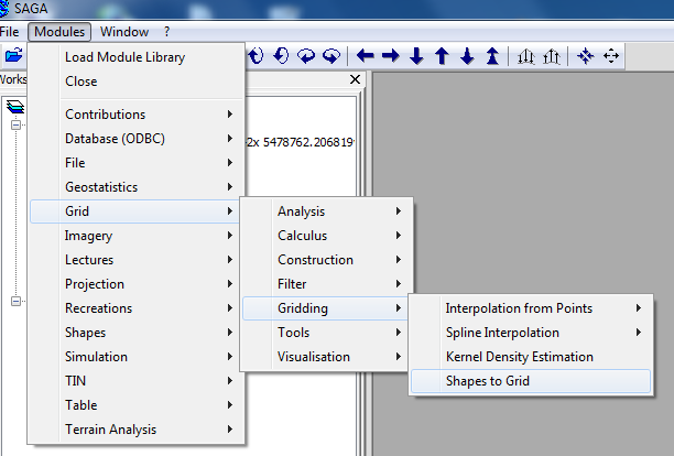
- First navigate to the Modules tab of the main menu toolbar.
- Open the Modules tab by clicking on it and then navigate down the drop down list to Grid.
- In the Grid menu that should have opened after you navigated to the Grid selection, you will need to find the Gridding toolset.
- In this toolset go down the list to the Shapes to Grid tool and open it.
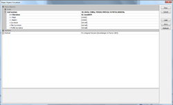
- The tool dialogue box will now open with many input options.
- The first two rows of the tool are labelled Shapes and Attribute and these options give the user the fields in which the vector polygon file that needs to be converted must be specified. So in the first row you will need to use the drop down menu and select the vector polygon file that needs to be converted. For this project the Okanagan Lake vector polygon was selected.
- In the second row you will need to select the attribute of the vector file that will determine the file outline boundaries. Note: because the file is just being converted in this case for the watershed delineation the any attribute can be chosen, and in this project the Object ID field was employed.
- The next row titled Method for Multiple Values you will need to select the Mean option from the drop down menu. This tells the conversion algorithm to take the average if two or more alike values are found in the vector file.
- The field called Method for Lines can be specified however you want. It just means that the outline of your vector polygon will either be thick or thin. For this project the thin option was employed.
- Preferred Target Grid Type field will vary depending on the type of vector data file you have. In this project the vector polygon for Okanagan Lake was a 8 byte vector and so the Floating Point (8 byte) option was chosen.
- The last field Target Grid needs to be set to Grid so that SAGA knows that a new grid needs to be created.
- The Shapes to Grid tool can be seen below to help you better understand the procedures.
- Once you have input all the required parameters for the tool click Okay and your vector polygon hydrologic feature will become a raster. Below the Okanagan lake raster is shown after being converted from a vector polygon.
Creating a Watershed map
This section will run through the actual hydrological analysis of generating watershed maps for a region. In this specific tutorial the Okanagan Lake watershed is generated only, but the procedures would apply to any study region. To make a watershed map:
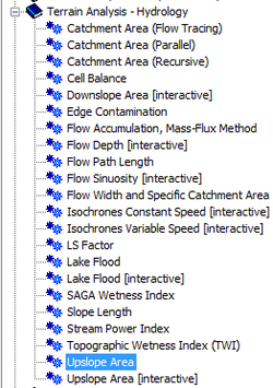
- Go to the workspace window's Modules Tab and scroll down to Terrain Analysis - Hydrology and expand it.
- Scroll down to Upslope Area and open the tool by double clicking.
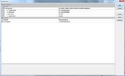
- Select your grid system through the drop down menu on the right side of the window on the Grid System row .
- Go down to the row titled Target Area and select your area of interest, which is the converted vector hydrologic feature on which the watershed will be based. In this tutorial the Target Area is the Okanagan Lake boundary raster file.
- Go down to the Elevation row and select your Filled DEM data from the drop down menu on the right side of the window.
- Ensure that the row titled Sink Routes has [not set] selected through the drop down menu. This field is specified as [not set] because the filled DEM already accounts for the sink routes of the data.
- Go down to the row titled Upslope Area and make sure [create] is selected in the drop down menu. This is the field that tells the algorithm to output the the watershed map which is also known as an upslope area map.
- Go under Options and to the row titled Method and make sure Deterministic 8 is selected from the drop down menu. Note: The Deterministic 8 (D8) algorithm is chosen in this project because it is found to be the best option when generating watershed maps. This D8 algorithm assumes that each cell of the Filled DEM has unidirectional water flow, whereas the other algorithms assume that one cell can have water flowing in multiple directions. To make a more accurate and understandable watershed delineation map the D8 algorithm is best.
- Now the next field is titled Convergence and for this row it is advised that you please ignore the field and leave the default value. It is important to leave the field untouched because this convergence factor only applies it you are using the multiple flow direction algorithm but because we have use the D8 algorithm this field will not apply to the output.
- After you have done all of the steps click Okay at the top right of the window.
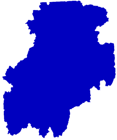
- This creates your Watershed Map.
Figure 6. Watershed of Lake Okanagan, British Columbia, Canada.
Now as seen in Figure 6 an excellent watershed delineation map has been generated for the study region, however you can also see that the watershed map is projected onto just a white background causing the information to be ambiguous and provide no geospatial meaning. In order for hydrologists and/or researchers in the real world to use this map successfully you would definitely need to drape this map over an other map (like a DEM, Basemap of the study region or aspect map) that provides geospatial context to the information so that researchers can actually see which areas of the study region contribute water flow into Okanagan Lake. In this project the watershed was given geospatial context by draping it over the aspect map because this map clearly depicts the landscape of the study region and help pinpoint areas that contribute water flow to the target area.
Figure 7. Watershed of Lake Okanagan, British Columbia, Canada shown draped over the aspect map in order to make the data more meaningful.
In Figure 7 you can see the watershed map draped over the aspect map. To drape the watershed over other maps you first need to convert the raster watershed file into a vector polygon and to do this:
- You will first need to open the tool called Vectorising Grid Classes by navigating through the menus of the main toolbar using the following steps: Modules | Shapes | Grid | Vectorization | Vectorising Grid Classes.
- Once the tool's dialogue box has opened you will need to once again select your grid system from the drop down list of the respective row.
- Next go down to the Grid field and input the Upslope Area map that was created for the watershed map.
- In the field titled Polygons may sure that the selection column is set as [create] so that the algorithm knows that a vector polygon needs to be generated.
- The next field called Class selection should be set as All Classes and the class identifier should be set as 1. This field will specify how many classes you want generated in the output vector polygon.
- The last input field called Vectorised class as... should be set to one single (multi-)polygon object because we want only one single polygon created. The other option of this field would create a vector file of the upslope area but with lots of polygons to build it, and using the one single option you will get one polygon which want is needed to drape it over the aspect map.
- Now click Okay and a new vector file will be generated of the watershed map.
The above steps describe the steps required to convert a raster to vector polygon so that the watershed map can be draped over the aspect map. Once the watershed map has been vectorised further steps can be taken to drape it over other maps for geospatial context. To do this:
- Go to the Data tab of the workspace window and find the upslope area vector polygon file.
- Click on the name of the file to select it and when it is highlighted go to the properties window which located on the right hand side of the screen.
- In the properties window ensure that you are in the Settings and then navigate to up to the field titled Transparency [%].
- In this field you can input any value you prefer based on how transparent you would like your watershed map to look when it is displayed over the aspect map. For the Okanagan Lake study area a transparency of 40 of selected.
- Once the transparency percentage has been specified click Apply and then Save at the bottom of the properties window.
- Now go back to the Data tab of the workspace window and right click on the watershed vector file.
- Select the Add layer to Map option.
- In the Map Selection Window that pops up select the Upslope area map.
- Finally click OK and now your Watershed map is fully completed and has great geospatial information along with its hydrological information just like Figure 7.
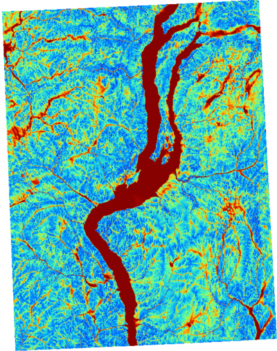
Creating a Wetness Index Map
This section will run through the analysis of defining a region's wetness, which describes how susceptible specific areas in a study region are to becoming saturated if high inputs of precipitation occur in a relatively short amount of time. To run a wetness index analysis conduct the following:
- In the workspace window under the Modules tab scroll down to Terrain Analysis - Hydrology' and expand it using the small plus sign button.
- Scroll down to SAGA Wetness Index tool and double click it to open the dialogue box to the analysis tool dialogue box.
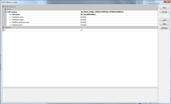
- Select your grid system through the drop down menu on the right side of the window on the Grid System row .
- Go down to the Elevation row and select your Filled DEM data from the drop down menu in the empty column beside the row title.
- Ensure Catchment area, Catchment slope, Modified catchment area and Wetness index all have [create] in each of the row's drop down menu of the window.
- In the row titled t make sure the row value is set to ten (10), since that is the default for the tool and it causes the wetness index values to being floating point numbers with a precision of ten points.
- After you have done this click Okay at the top right of the window.
- This creates your Wetness Index Map.
Figure 8. Map displaying the Wetness Index of the Lake Okanagan Region; where red shows highest wetness and blue shows driest areas.
Conclusion -- Completed Objectives
Better understand how the software works.
Steps need to be taken in order to achieve the desired output maps that are both accurate based on the input data and informative for the specific study region and hydrologic information.
References
USGS. (2013, May 23). What is hydrology and what do hydrologists do? Retrieved from The USGS Water Science School: http://ga.water.usgs.gov/edu/hydrology.html
V. Olaya, O. Conrad. (2009). Chapter 12 Geomorphometry in SAGA, Developments in Soil Science, Volume 33, Pages 293-308

