Enhanced Wetness Modelling in SAGA GIS

Purpose

The purpose of this tutorial is not only to present an efficient workflow for modelling wetness, but also to explain the different options offered for module inputs throughout the way, as well as why the chosen ones were favoured. The SAGA documentations show that different options are available, yet only includes a reference to a paper that tells where the method was derived from with minimal description. This tutorial will explain how the used methods work and what differentiates them from others. Other methods that were options but not used will be briefly explained as well.

Preamble

This is a workflow that offers an enhanced method for modelling wetness of a terrain. A terrain’s wetness index is a secondary terrain attribute derived from a digital elevation model through different transformations to the raster grid. The method presented in this tutorial is rather more detailed and precise then others because the two defining parameters involved in calculating a wetness index (up slope area and slope) are calculated in particular ways that do not use the assigned defaults or the one step algorithms.

Attention: this workflow has been generated using SAGA GIS 2.2.2 thus all the headings and toolset names are specific to this version. Slight differences in module names are introduced between this version and the one before. SAGA offers Module Library Documentations for the last 5 version. Note that some instructions that yield the same result might have different names/options in different versions (e.g. Catchment Area tool in 2.2.2 was called Flow Accumulation in 2.1.2). Another helpful resource would be the SAGA Forum where a lot of resources and exchanges between GIS users are available.

SAGA GIS was used because of its high efficiency in processing spatial data, and its many offered options for dealing with environmental modelling. SAGA GIS is also a Free Open Source Software (FOSS) which means its source code can be manipulated to suit the user’s needs. In this tutorial no custom code or automation was used, but would be considered for a bigger workflow to increase productivity. To download SAGA GIS: http://sourceforge.net/projects/saga-gis/files/

Introduction to the SAGA Environment

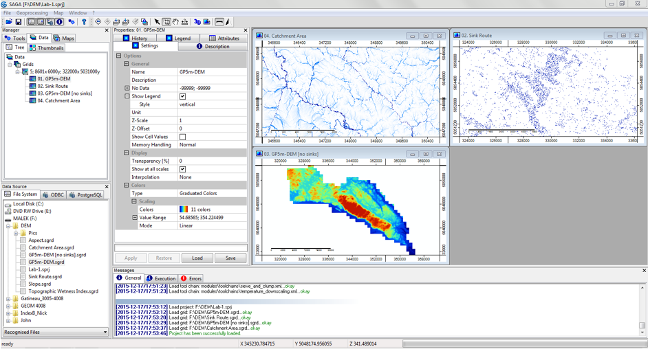
Throughout your work in SAGA GIS, the tools used, progress, errors, and results can be tracked in different ways. The figure below shows what the SAGA GIS workspace looks like. The main control sections are the Manager, Data Source, Properties, and Messages.

• For accessing folders and data files refer to Data Source | File System (left of the screen). The imported data will appear under Manager; once the data layer is double clicked, it will appear in the right part of the screen as a Map layer.
• Under Properties, information about the layer can be viewed, as well as settings, symbology, attributes, and history of processing.
• The bottom part of the screen has Messages which will show in the General tab every single command ran in SAGA with the time of execution and if the method succeeded or not.
• The Execution tab shows the inputs assigned to the module.
• If any errors arise during running, they appear under the Errors tab.
• To track the used tools as well, SAGA keeps a record of the last used tools in order under Geoprocessing.

Data & Study Site

This exercise is done using data from Gatineau Park, Quebec (Canada). The used data:

• Digital Elevation Model (DEM): LiDAR-derived, 5 meter resolution
• Gatineau Park boundary: polygon layer

The data used is acquired from a non-public source, however, any DEM can be used to execute the same workflow demonstrated by this tutorial.

Setting Environment

Data Import

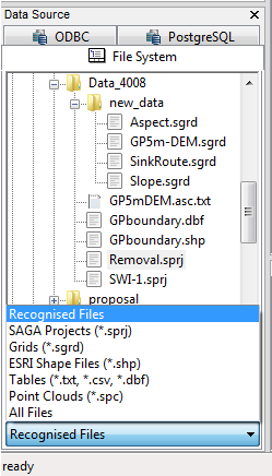
As mentioned above, to access and import layers into the SAGA workspace, the user’s working directory is displayed at the bottom left of the screen under File System. There, polygon, grid, and table data can be shown and imported if double clicked on. Other SAGA projects (*.sprj) can also be shown and launched with a double click.

• The DEM used in this project was acquired as a text file (*.txt) in ASCII format. Given that, double clicking on it will import it as a table and not a raster grid.
• To import the DEM as a raster grid, the geospatial data acquisition library GDAL is used. GDAL is a translator library that is usually coupled with another library OGR. GDAL is used to translate raster data formats into spatial software whereas OGR is for vector data translation and design.

• To import the ASCII DEM used, GDAL can be reached through: Geoprocessing |File |GDAL/OGR | GDAL: Import raster
• Locate your ASCII text file, and set the Interpolation to Nearest Neighbour.
• To import the boundary layer, as mentioned beforehand, just double click on GPboundary.shp (in File Systems).

Saving Data

Saving in SAGA has to be done manually. Any processed layer that is set to <create> and consequently added to the Data section is not automatically saved. That said, to save a created layer, right click on it and go to Save As.

Data Referencing

The following section deals with the Projection Module in SAGA GIS. If the data used is in the right and desired projection, skip to the next section.

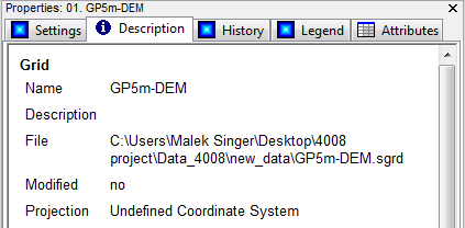
• In the Description of the DEM, we notice that once imported, it comes in with an Undefined Coordinate System.

• In order to have this layer with the correct coordinate reference system (CRS), we need to set the coordinate reference system that the data originally was created in and then transform the coordinates into the desired projection.
• We know that the original data’s projection was NAD 83 MTM 9 and thus we should set the CRS to that accordingly.
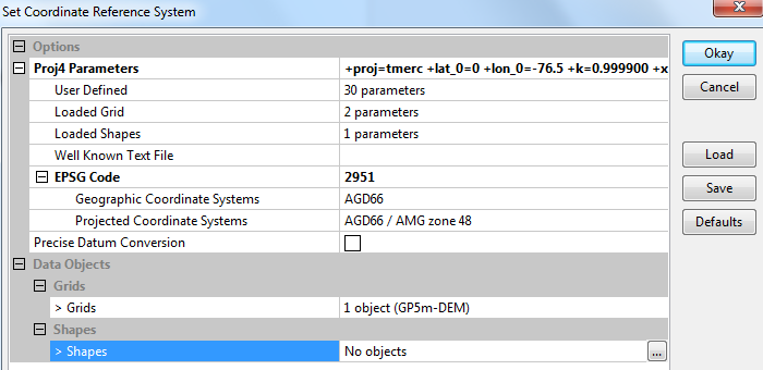
• To do that go to Geoprocessing | Projection | Set Coordinate system. The way this module is set up allows for extracting CRS information about the desired system from different sources. These methods include a Proj4 command line specific to that system, using a coordinate system of an already Loaded Grid, inputting an EPSG (a structured code for worldwide reference systems and transformations) code for that system, etc.
• In this example, we will be setting the EPSG of the MTM 9 projection. To retrieve that, visit http://spatialreference.org/ and search for NAD83 (CSRS) / MTM zone 9. The EPSG should be 2591.
• Under Options| EPSG Code paste 2591; this will automatically change the Proj4 Parameter up in the module.
• Under Grids select the imported DEM and hit Okay.

• Under the Description of the DEM, the Projection should no longer be Undefined Coordinate System but rather :

->Projected Coordinate System [EPSG 2951]:NAD83(CSRS)/MTMzone9[+proj= tmerc +lat_0=0 +lon_0=-76.5 +k=0.999900 +x_0=304800 +y_0=0 +ellps=GRS80 +units=m +no_defs ].

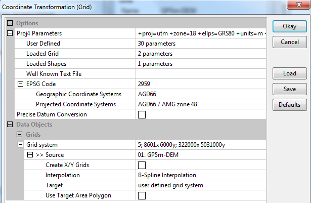
• Now that the original CRS was re-established, the desired projection of the workspace can be transformed to. To do that, go to Geoprocessing | Projection | Coordinate Transformation (Grid).
• Just like the previous step, look up the EPSG of NAD 83 and paste it in the EPSG section; assign the Grid to the used DEM, and leave everything else as default. Hit Okay.

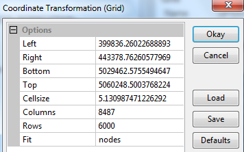
• Another window will pop up, it includes the extent of the layer as well as properties of the grid used. Make sure to resample the cell size to whatever the input DEM resolution is. In the used DEM, it is 5 meters.

• The final DEM should now be in UTM 18N (NAD83 CSRS)->Projected Coordinate System [EPSG 2959]: NAD83 (CSRS)/UTMzone18N [+proj=utm +zone=18 + ellps=GRS80 +units=m +no_defs ]

Clipping

The original DEM used is slightly bigger than the actual area of Gatineau Park. This is probably due to the stitching of tiles and the interpolation method of point clouds. That said, for a more appropriate cartographic result, using the Gatineau Park boundary layer which is a polygon format, the output rasters will be clipped. To do that Geoprocessing | Shapes| Grid | Spatial Extent | Clip Grid with Polygon

Data Modelling

Topographic Wetness Index abstract

The topographic wetness index, coined by Beven and Kirkby in 1979, aims to quantify the influence of topography on hydrological processes within a watershed. In its basic form, it works by deriving slope and accumulation distribution parameters from a topographic model (Sørensen et al., 2006) and then feeds them into the following relation:

-->TWI= ln[(upstream area)/tan(Slope)] where TWI is the topographic wetness index.

In order to compute the TWI, the upstream area and the slope are needed.

Slope Derivation

The description of how the methods work are in reference to Zevenbergen, L.W., Thorne, C.R. (1987):'Quantitative analysis of land surface topography', Earth Surface Processes and Landforms, 12: 47-56.

• The computation of a slope parameter in a GIS environment is usually considered a trivial one-step algorithm that outputs visually appealing rasters. In SAGA GIS however, there are multiple methods for the calculation of slopes based on different considerations of geometry, polynomial order, and scale.

• SAGA offers 8 different options for calculating slope:
  • Maximum slope (Travis et al. 1975)
  • Maximum triangle slope (Tarboton 1997)
  • Least squares fitted plane (Horn 1981, Costa-Cabral & Burgess 1996)
  • 6 parameter 2nd order polynomial (Evans 1979)
  • 6 parameter 2nd order polynomial (Heerdegen & Beran 1982)
  • 6 parameter 2nd order polynomial (Bauer, Rohdenburg, Bork 1985)
  • 9 parameter 2nd order polynomial (Zevenbergen & Thorne 1987)
  • 10 parameter 3rd order polynomial (Haralick 1983)

• The used method is the one proposed by Zevenbergen & Thorne (1987) which is the 9 parameter 2nd order polynomial where slope is the first derivative of elevation.
  • It uses a rectangular matrix of evenly spaced elevations that covers the entire area of the input layer where elevation points are used to determine the parameters in the quadratic equation. In other words, equation fitting is used to map out the surface and derive different indices (slope, aspect, curvature, etc.)
  • This method uses an equation with 9 parameters to resolve for indices. It is more general than the other methods using 6 and more flexible (if a surface is of lower order than the equation, the corresponding coefficients will equal zero and wont influence the equation).
  • Many of the applications of this method pertain to hydraulic sediment transport which requires a slope to be dimensionless; the output is a dimensionless slope (although has the option for choosing a unit, for transport calculations, this slope is not restrained to a unit).
  • An advantage of this method is also the fact that it not only is able to yield an up slope area (drainage area contributing to a pixel) but also an up slope distance (longest travel path to an up slope divide).
  • The first three methods are focused on flow routing logic, operate on a local scale basis and have a particular restriction because they calculate slope in a uni-directional way from one cell to the other and thus would be fine for a simplistic wetness model but not this one.

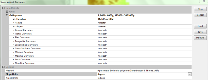
In order to compute for slope go to: Geoprocessing | Terrain Analysis | Morphometry | Slope, Aspect, Curvature

• Set the grid to the one we’ve been using throughout the workflow, and the inputted DEM.
• Make sure Slope and Aspect are set as <create>. For the purposes of this workflow we are not totally interested in curvature models so leave them as <not set> (they look cool so feel free to play with them!).

• Make sure that the selected method is 9 parameter 2nd order polynom (Zevenbergen & Thorne 11987) and that the slope units is in degrees).

Catchment Area

Sink Drainage Route Detection

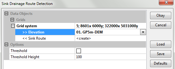
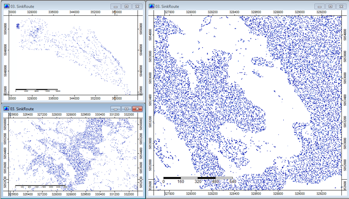
This method is used to correct for dips and sinks inherent in the DEM. The algorithm works by identifying sinks or pits in the digital terrain and the direction that water flows out of the sink (Cimmery, 2010). Such sinks are usually depressions in the DEM that are lower than their surrounding pixels which introduce error while using flow routing algorithms in hydrological analysis. The method outputs a “Sink Route” layer. -->Geoprocessing | Terrain Analysis |Preprocessing | Sink Drainage Route Detection.

The method will take the DEM as an input only. Make sure that Sink Route is set to <create> and that everything else is default. For the purposes of this exercise, setting a threshold in not necessary. A threshold in this method and the one after is the elevation at which the method will not fill a sink beyond. In other words, if a certain cratered geologic surface is of interest, but a fill is required to correct for sinks, the user might want to set a threshold of 50 where craters 50 meters in depth will not be filled.

Sink Removal

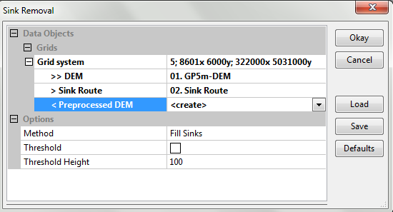
Now that the sinks are identified, they can be removed. There are multiple ways of “leveling” the sinks in the landscapes in SAGA’s Preprocessing toolbox. These include Fill Sinks (Planchon/Darboux, 2001), Fill Sinks and Fill Sinks XXL (Wang Liu), Flat Detection and Sink Removal.

All of the mentioned methods only require the DEM as an input parameter and return a filled one except the Sink Removal method. The method takes in an optional Sink Route parameter which yields a finer result because it takes into consideration sink location and spill direction. Geoprocessing | Terrain Analysis |Preprocessing | Sink Removal The input being the DEM, and Sink Route. Make sure to set Preprocessed DEM as <create>.

Catchment Area calculation

The details mentioned in this section are in reference to (Cimmery, 2010) In their basic forms, catchment area methods use a flow accumulation algorithm that saturates a pixel depending on how many pixels upstream (area wise) lead into it across a topographic/directional gradient. The logic that determines how flow is transferred from one pixel to the other however is very variable and yield highly distinctive results.

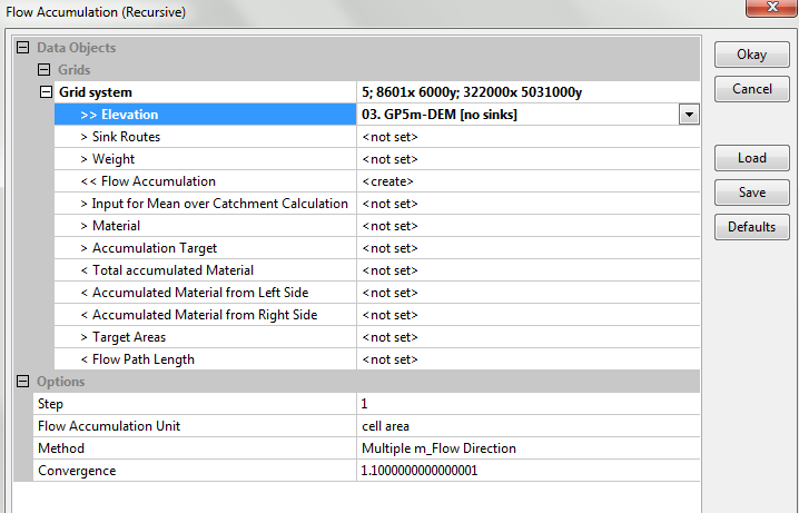
The catchment area algorithm used in this workflow is recursive. This means it takes in the filled DEM and recursively processes all upward connected pixels until all pixels have been processed and a value is computed. The computation of the area/accumulation value is selected to be done through a Multiple Flow Direction method. The available options for flow accumulation method are D8, D Infinity, and Modified Flow Distribution.

• D8: flow goes between cell centres across an elevation gradient to where the steepest neighboring cell is detected. The flow of water is to the neighboring cell with the lowest elevation (i.e. the steepest gradient). The direction of flow however is restricted to multiples of 45º which introduces a lot of flow constraints and thus is not always favourable.
• D Infinity: modified and more accurate method than D8, yet can still only allow flow to be divided to the two most favourable cells. In more technical words, “The method is based on representing flow direction as a single angle taken as the steepest downwards slope on the eight triangular facets centered at each grid point. The flow is then proportioned between two down-slope cells according to how close this flow direction is to the direct angle to the down-slope cell (Tarboton, 1997).” (Cimmery,2010)
• MFD: this method computes the flow distribution with divergence. This means that instead of a total flow from one cell to the other based on gradient steepness, flow is distributed based on slope-weight basis and thus fractions of the flow are passed to neighboring cells differentially. This yields a more accurate representation of flow in variable terrain.

To run this method, Geoprocessing | Terrain Analysis | Hydrology | Flow Accumulation | Flow Accumulation (Recursive)

File:Catchementrecursive