Difference between revisions of "Generating Wetness Indices for Watersheds in GRASS"
| (120 intermediate revisions by 39 users not shown) | |||
| Line 1: | Line 1: | ||
=Introduction:= |
=Introduction:= |
||
| − | In hydrology, a watershed refers to an area of land in which all the precipitation runoff drains into a common waterway, such as a lake, river, or ocean. |
+ | In hydrology, a watershed refers to an area of land in which all the precipitation runoff drains into a common waterway, such as a lake, river, or ocean. In other words, watersheds act as natural funnels, collecting the precipitation that lands within their borders, and directing it into the common waterway outlet. Watersheds are arranged in hierarchical order, where the size of a given watershed is determined by the location of its outlet. Thus, as the outlet of a watershed moves downstream, the watershed becomes larger and consists of more sub-watersheds. In hydrology, watersheds are extremely important since they delineate regions that contribute to flow in a given waterway. |
| − | Wetness indices are used to describe spatial moisture patterns within a given region. They are calculated based on a region’s contributing upslope area |
+ | Wetness indices are used to describe spatial moisture patterns within a given region. They are calculated based on a region’s slope and contributing upslope area, where areas with low slope and large contributing area are expected to be relatively wet and areas with high slope and small contributing area are expected to be relatively dry. When a wetness index is calculated for a given region, the index should be calculated for the entire watershed in which that region is located, in order to ensure accuracy in the 'contributing upslope area' parameter. |
| + | =Procedure:= |
||
| + | This exercise was originally written for use by Carleton University for the purpose of providing a learning tool in the Department of Geography and Geomatics, under the course code GEOM 4008. The first version was written in 2010, and it was checked and updated in 2017. The updated screenshots seen below are from a Windows 7 Operating System. If you do not currently have these programs on your desktop please see the following links: For Quantum GIS download: [http://www.qgis.org/en/site/forusers/download.html] For GRASS GIS download: [https://grass.osgeo.org/download/] |
||
=Outline:= |
=Outline:= |
||
| − | This tutorial illustrates the processes involved in delineating watershed boundaries, as well as generating topological wetness indices inside those boundaries. These processes will be performed using GRASS tools through Quantum GIS. The tutorial also discusses the effects of filtering DEMs on wetness indices |
+ | This tutorial illustrates the processes involved in delineating watershed boundaries, as well as generating topological wetness indices inside those boundaries. These processes will be performed using GRASS tools through Quantum GIS. The tutorial also discusses the effects of filtering DEMs on wetness indices and introduces a means of verifying both watershed boundaries and wetness index images. |
| − | Images from a sample analysis are also provided for each step |
+ | Images from a sample analysis are also provided for each step described in the tutorial. In the sample analysis, the Carp River watershed in Ottawa, Ontario is delineated, and a wetness index is generated for the watershed region. A DEM of the Ottawa-Gatineau region, with 50m cell size, was used for the sample analysis. |
| Line 18: | Line 20: | ||
=Setting Up Your Workplace= |
=Setting Up Your Workplace= |
||
1. In QGIS, open the DEM using the 'Add Raster Layer' button in the 'Manage Layers' toolbar. |
1. In QGIS, open the DEM using the 'Add Raster Layer' button in the 'Manage Layers' toolbar. |
||
| + | |||
| + | [[File:Addraster.jpg]] |
||
2. Once the DEM is loaded in QGIS, create a new GRASS mapset with an appropriate projection and workplace extent. |
2. Once the DEM is loaded in QGIS, create a new GRASS mapset with an appropriate projection and workplace extent. |
||
| Line 23: | Line 27: | ||
3. Using r.in.gdal.qgis, import the DEM into the new mapset. |
3. Using r.in.gdal.qgis, import the DEM into the new mapset. |
||
| + | [[File:Uploadingtool.png|500px]] |
||
| − | |||
=Generating Watershed Boundaries:= |
=Generating Watershed Boundaries:= |
||
| Line 29: | Line 33: | ||
==''r.watershed''== |
==''r.watershed''== |
||
| − | + | * This method is designed for analysis in which the delineation of all watersheds over a specified size is required. |
|
| − | + | * If a watershed with a ''specific outlet point'' is required, use the r.water.outlet module. |
|
| Line 37: | Line 41: | ||
1. Open the ''r.watershed'' module. |
1. Open the ''r.watershed'' module. |
||
| + | |||
| + | [[File:Rwatershed.png|400px]] |
||
2. Select the DEM as the input map. |
2. Select the DEM as the input map. |
||
| − | 3. Select a proper input value. The input value (or threshold in command line) refers to the minimum size in image pixels a watershed must contain |
+ | 3. Select a proper input value. The input value (or threshold in the command line) refers to the minimum size in image pixels a watershed must contain to be delineated. |
| + | |||
| + | [[File:Watershed1.PNG|400px]] |
||
4. Specify a name for 'Output Map: Unique label for each watershed basin'. |
4. Specify a name for 'Output Map: Unique label for each watershed basin'. |
||
| − | Alternatively, this can be done in command line |
+ | Alternatively, this can be done in the command line: |
| + | :r.watershed elevation=DEM threshold=# basin=Watersheds |
||
| − | - This watershed output image will include ''all'' watersheds that exist within the DEM, given the threshold parameter that was specified. |
||
| − | - Each watershed in the image is assigned a unique pixel value. |
||
| + | * This watershed output image will delineate ''all'' watersheds that exist within the DEM, given the threshold parameter that was specified. |
||
| + | * Each watershed in the image is assigned a unique pixel value. |
||
| − | ===Watershed Masks:=== |
||
| − | Since this method produces a watershed map consisting of numerous watersheds, if analysis on a particular watershed is required, a watershed mask is often required. |
||
| + | '''Watershed Masks:''' |
||
| − | A watershed mask can be produced in command line based on: ''[r.mapcalc WatershedMask=if (Watersheds==’unique watershed label’]'' |
||
| + | Since this method produces a watershed map consisting of numerous watersheds, if analysis on a particular watershed is required, a watershed mask will also be required. |
||
| − | In the mask, areas within the watershed are assigned a value of 1, and all other areas are assigned a value of 0. |
||
| + | [[File:Findingmapcalc.png|400px]] |
||
| + | |||
| + | [[File:MapcalcAF.PNG|400px]] |
||
| + | |||
| + | A watershed mask can be produced in command line based on: |
||
| + | :r.mapcalc WatershedMask=if (Watersheds==’unique watershed label') |
||
| + | |||
| + | In the mask, areas within the watershed are assigned a value of 1, and all other areas are assigned a value of 0. |
||
==''r.water.outlet''== |
==''r.water.outlet''== |
||
| − | + | * Unlike r.watershed, this method will delineate a watershed based on the coordinates of its outlet point. |
|
| − | + | * This allows practitioners to customize the scale of output watersheds based on their research needs, without having to tamper with a threshold parameter. |
|
| Line 68: | Line 83: | ||
1. Open the r.watershed module. |
1. Open the r.watershed module. |
||
| + | |||
| + | [[File:Rwatershed.png|400px]] |
||
2. Select the DEM as the input map. |
2. Select the DEM as the input map. |
||
| Line 73: | Line 90: | ||
3. Specify a name for 'Output Map: Drainage Direction'. |
3. Specify a name for 'Output Map: Drainage Direction'. |
||
| − | + | * The output image quantifies the drainage direction of cells throughout the DEM. |
|
4. Open the r.water.outlet module. |
4. Open the r.water.outlet module. |
||
| + | |||
| + | [[File:Rwateroutlet.png|400px]] |
||
5. Select the Drainage Direction map as 'Name of Input Raster Map'. |
5. Select the Drainage Direction map as 'Name of Input Raster Map'. |
||
| + | |||
| + | [[File:Watershed2.PNG]] |
||
6. Specify the easting and northing of the watershed outlet point in 'The Map E Grid Coordinates' and 'The Map N Grid Coordinates'. |
6. Specify the easting and northing of the watershed outlet point in 'The Map E Grid Coordinates' and 'The Map N Grid Coordinates'. |
||
| Line 85: | Line 106: | ||
Alternatively, this can be done in command line based on: |
Alternatively, this can be done in command line based on: |
||
| − | + | ::r.watershed elevation=DEM drainage=DrainageDirection |
|
| − | + | ::r.water.outlet drainage=DrainageDirection basin=Watersheds easting=x northing=y |
|
| − | + | * The watershed output image will only include the watershed for which the outlet point was specified. |
|
| − | + | * The watershed output image is essentially a mask of the watershed. |
|
| Line 95: | Line 116: | ||
[[File:WatershedsComp.png|800px]] |
[[File:WatershedsComp.png|800px]] |
||
| − | ''Figure 2: Left: The watershed boundaries generated in r.water.outlet, using x,y coordinates obtained from a topographic map |
+ | ''Figure 2: Left: The watershed boundaries generated in r.water.outlet, using x,y coordinates obtained from a topographic map.'' |
| + | ''Right: The watershed boundaries generated in r.watersheds, using a threshold parameter of 10000.'' |
||
| − | |||
=Generating Wetness Indices:= |
=Generating Wetness Indices:= |
||
| Line 106: | Line 127: | ||
1. Open the r.slope.aspect.slope module. |
1. Open the r.slope.aspect.slope module. |
||
| + | |||
| + | [[File:Slope aspect.png|400px]] |
||
2. Select the DEM for ‘Name of Elevation Raster Map’. |
2. Select the DEM for ‘Name of Elevation Raster Map’. |
||
| + | |||
| + | [[File:Slopeopen.PNG|400px]] |
||
3. Specify a name for ‘Name for Output Slope Raster Map’. |
3. Specify a name for ‘Name for Output Slope Raster Map’. |
||
| + | |||
| + | [[File:Slopeopen2.PNG|400px]] |
||
| − | Alternatively, this can be done in command line based on |
+ | Alternatively, this can be done in command line based on: |
| + | ::r.slope.aspect elevation=DEM slope=Slope format=degrees |
||
| − | + | * The slope output image reports the slopes of the DEM landscape in degrees or percent slope, according to the user's choice. |
|
| − | - The slope image will commonly contain regions where slope equals zero. |
||
| − | - Since slope appears in the denominator of the wetness index equation, zero slope areas will result in undetermined (null) regions in the output wetness index maps. |
||
| + | * The slope image will commonly contain regions where slope equals zero. |
||
| + | * Since slope appears in the denominator of the wetness index equation, zero slope areas will result in undetermined (null) regions in the output wetness index maps. |
||
| + | |||
| − | ===Eliminating Zero Slope Areas in Slope Maps:=== |
||
| + | '''Eliminating Zero Slope Areas in Slope Maps:''' |
||
| − | To avoid null values in the wetness index image, zero slope areas in the output slope images should be assigned a value of 0.0001 (or any other very small value). |
||
| + | |||
| + | To avoid null values in wetness index images, zero slope areas in output slope images should be assigned a value of 0.0001 (or any other very small value). |
||
| Line 126: | Line 156: | ||
1. Open the r.mapcalculator module. |
1. Open the r.mapcalculator module. |
||
| + | |||
| + | [[File:Findingmapcalc.png]] |
||
2. Select the output slope map as ‘A’. |
2. Select the output slope map as ‘A’. |
||
| Line 136: | Line 168: | ||
Alternatively, this can be done in command line based on [r.mapcalc Slope_NoZeros = Slope + 0.0001] |
Alternatively, this can be done in command line based on [r.mapcalc Slope_NoZeros = Slope + 0.0001] |
||
| − | + | * This will replace zero slope values with slopes of 0.0001. |
|
| − | + | * The increase in slope in all other areas is negligible. |
|
| − | |||
| − | |||
| − | [[File:Slope1.png|600px]] |
||
| − | |||
| − | ''Figure 3: The output slope image and the user-defined color rules that were used to display the image.'' |
||
| − | |||
==Upslope Contributing Area:== |
==Upslope Contributing Area:== |
||
| Line 152: | Line 178: | ||
1. Open the r.watershed module. |
1. Open the r.watershed module. |
||
| + | |||
| + | [[File:Rwatershed.png|400px]] |
||
2. Select the DEM as the input map. |
2. Select the DEM as the input map. |
||
| Line 158: | Line 186: | ||
| − | Alternatively, this can be done in command line based on |
+ | Alternatively, this can be done in command line based on : |
| + | :r.watershed elevation=DEM accumulation=AccumFlow |
||
| − | + | * The output image quantifies the number of cells that drain through each cell or, in other words, the number of cells that are upslope from a given cell. |
|
| Line 169: | Line 198: | ||
1. Open the r.mapcalculator module. |
1. Open the r.mapcalculator module. |
||
| + | |||
| + | [[File:Findingmapcalc.png|400px]] |
||
2. Select the flow accumulation image as ‘A’. |
2. Select the flow accumulation image as ‘A’. |
||
| Line 182: | Line 213: | ||
[[File:AccumFlow1.png|600px]] |
[[File:AccumFlow1.png|600px]] |
||
| − | ''Figure 4: The output accumulated flow image and the user-defined color rules that were used to display the image |
+ | ''Figure 4: The output accumulated flow image and the user-defined color rules that were used to display the image.'' |
| + | Although the upslope contributing area is used to calculate wetness index, accumulated flow is illustrated in Figure 4 due to a time constraint. However, due to the nature of the upslope contributing area, the two images appear exactly the same. |
||
==Wetness Index:== |
==Wetness Index:== |
||
| Line 192: | Line 224: | ||
1. Open the r.mapcalculator module. |
1. Open the r.mapcalculator module. |
||
| + | |||
| + | [[File:MapcalcAF.PNG|400px]] |
||
2. Select the upslope contributing area image as ‘A’. |
2. Select the upslope contributing area image as ‘A’. |
||
| Line 202: | Line 236: | ||
| − | Alternatively, this can be done in command line based on |
+ | Alternatively, this can be done in command line based on: |
| − | + | ::r.mapcalc WetnessIndex = log(UpslopeContArea/tan(Slope), 2.718282) |
|
| Line 211: | Line 245: | ||
| − | + | '''Standardizing Wetness Index Maps:''' |
|
| + | |||
A common approach when comparing wetness indices is to standardize values between 0-1. If output wetness index images are going to be compared with other indices, standardize index values using r.mapcalc and r.info. |
A common approach when comparing wetness indices is to standardize values between 0-1. If output wetness index images are going to be compared with other indices, standardize index values using r.mapcalc and r.info. |
||
| + | [[File:Findingrinfo.png|400px]] |
||
| − | Standardizing images can be done in command line based on [r.mapcalc StandardizedImage= ((Image – ImageMin)/(ImageMax – ImageMin))]. |
||
| + | Standardizing images can be done in command line based on [r.mapcalc StandardizedImage= ((Image – ImageMin)/(ImageMax – ImageMin))]. |
||
=Displaying Maps:= |
=Displaying Maps:= |
||
| − | Given the extremely large flow values in creeks, streams, and tributaries within the watershed, flow accumulation images are often hard to interpret without user-defined color rules. |
+ | Given the extremely large flow values in creeks, streams, and tributaries within the watershed, flow accumulation and upslope contributing area images are often hard to interpret without user-defined color rules. Slope and wetness index images also required user-defined color rules for proper visual display. |
| − | To generate user-defined color rules: |
||
| + | To display images based on user-defined color rules: |
||
| − | 1. Obtain the distributions for values in the image using: |
||
| − | \tA. r.stats –c FileName – returns counts for each value that exists in the image. |
||
| − | \tB. QGIS Histogram function. |
||
| + | 1. Generate distributions for an image using the ''r.stats –c '' module in GRASS or the ''Histogram'' function in QGIS. |
||
| − | 2. Based on the distributions, determine suitable color breaks for the color rules. |
||
| + | 2. Based on the distribution and your research needs, determine suitable color breaks for displaying the image. |
||
| − | 3. Create color rules in a text file (.txt) based on: |
||
| + | 3. Create a text file (.txt) containing the color rules for the image. |
||
| − | [[File:ColorRules.png]] |
||
| + | Refer to [http://grass.fbk.eu/grass62/manuals/html62_user/r.colors.html r.colors] for syntax of color rules. |
||
| − | To apply user-defined color rules: |
||
| − | + | 4. Open the r.colors module. |
|
| + | [[File:Findingrcolours.png|400px]] |
||
| − | 2. Select the image in ‘Name of Input Raster Map’. |
||
| + | 5. Select the image in ‘Name of Input Raster Map’. |
||
| − | 3. Specify the full path to user-defined color rules text file in the ‘Path to Rules File’ browser. |
||
| + | [[File:Workingrcolours.PNG|400px]] |
||
| − | Alternatively, this can be done in command line based on [r.colors map=FlowAccum rules=‘FullPathToColorRules’] |
||
| + | 6. Specify the full path to user-defined color rules text file in the ‘Path to Rules File’ browser. |
||
| − | =DEM Filtering:= |
||
| − | In order to achieve a specific level of detail in final wetness index images, filtering the DEM prior to generating the slope and flow accumulation maps may be required. Filtering can also reduce errors in future output maps that are caused by the DEM, or how the DEM was created. |
||
| + | Alternatively, this can be done in command line based on: |
||
| − | Although slope, flow accumulation and wetness index can be filtered directly after output, by limiting filtering to the DEM only, all output maps are known to be derivatives of a specific elevation model. In other words, by limiting filtering to the DEM, it is very clear which DEM the maps are reporting slope, flow, or wetness for. |
||
| + | ::r.colors map=FlowAccum rules=‘FullPathToColorRules’ |
||
| + | =DEM Filtering:= |
||
| − | In this analysis, a total of four wetness indices were generated for the Carp watershed, each generated from a DEM filtered by a 5x5 average filter a varying number of times. All indices were generated using the methodologies described in this tutorial. The indices were generated based on four DEMs that were filtered 0 times, 5 times, 10 times and 15 times prior to generating slope and flow accumulation images. |
||
| + | So far, all sample analysis images that are illustrated were generated from an unfiltered DEM. However, in order to achieve a specific level of detail in final wetness index images, filtering the DEM prior to generating the slope and flow accumulation maps may be required. Filtering can also reduce errors in future output maps that are caused by the DEM, or how the DEM was created. The DEM should be the only image that is filtered throughout the analysis. This ensures that all output images are derivatives of a specific elevation model. However, filtering final output maps '''for visual display''' is acceptable. |
||
| + | |||
To apply a filter to a DEM: |
To apply a filter to a DEM: |
||
| − | 1. Create a filter file which contains the |
+ | 1. Create a filter file which contains the filter you have chosen. |
| − | + | * In the sample analysis, the filter file contained a single 5x5 average filter; however, multiple filters can be included in one filter file. |
|
| + | * Refer to [http://grass.osgeo.org/gdp/html_grass64/r.mfilter.html r.mfilter] for the syntax of filter files. |
||
| − | |||
| − | - In the sample analysis, the filter file was as follows: |
||
| − | |||
| − | [[File:FilterFile.png]] |
||
2. Open the r.mfilter module. |
2. Open the r.mfilter module. |
||
| + | |||
| + | [[File:Findingrmfilter.png|400px]] |
||
3. Select the DEM in ‘Name of Input Raster Map’. |
3. Select the DEM in ‘Name of Input Raster Map’. |
||
| + | |||
| + | [[File:Mfilter1.PNG|400px]] |
||
4. Specify a name for ‘Name of Output Raster Map’. |
4. Specify a name for ‘Name of Output Raster Map’. |
||
| Line 271: | Line 307: | ||
6. Specify the number of times to repeat the filter. |
6. Specify the number of times to repeat the filter. |
||
| + | |||
| + | [[File:Mfilter2.PNG|400px]] |
||
Alternatively, this can be done in command line based on [r.mfilter input=DEM output=DEM_filtered filter= ‘path to filter file’ repeat= ‘number of repeats’]. |
Alternatively, this can be done in command line based on [r.mfilter input=DEM output=DEM_filtered filter= ‘path to filter file’ repeat= ‘number of repeats’]. |
||
| − | |||
| − | Images are provided from each output wetness index, to allow investigation of the differences in wetness index output resulting from filtering the DEM with a 5x5 average filter. Generally trial and error is required to find the proper series of filters for your research needs. However, the following images should give an idea on the basic effects of average filtering. |
||
| + | In the sample analysis, a total of four wetness indices were generated for the Carp watershed. All indices were generated using the methodologies described in this tutorial. Each was generated from a DEM that was filtered by a 5x5 average filter a varying number of times. The DEMs were filtered 0 times, 5 times, 10 times and 15 times prior to generating wetness index images. Screenshots of each wetness index are provided to allow an investigation into changes in wetness index that result from changes in DEM filtering processes. |
||
| − | [[File:WetnessIndexComparison.png]] |
||
| + | Although these screenshots will convey the general effects of DEM filtering, trial and error will likely be required to find the proper series and types of filters for your research needs. |
||
| − | Figure 6: Wetness indices that were generated from differently filtered DEMs. |
||
| − | [[File: |
+ | [[File:WetnessIndexComparison.png|600px]] |
| − | Figure |
+ | ''Figure 6: Wetness indices that were generated from a differently filtered DEM.'' |
| + | ''[Top Left: Unfiltered, Top Right: 5x5 filter x5 times, Bottom Left: 5x5 filter x10 times, Bottom Right: 5x5 filter x15 times]'' |
||
| − | [[File: |
+ | [[File:NorthernWetnessIndices.png|850px]] |
| − | Figure |
+ | ''Figure 7: Wetness indices generated from differently filtered DEMs, superimposed on topographic maps during verification.'' |
| + | ''[A: Unfiltered, B: 5x5 filter x5 times, C: 5x5 filter x10 times, D: 5x5 filter x15 times]'' |
||
| + | |||
| + | [[File:SouthernWetnessIndices.png|850px]] |
||
| + | |||
| + | ''Figure 8: Wetness indices generated from differently filtered DEMs, superimposed on topographic maps during verification.'' |
||
| + | ''[A: Unfiltered, B: 5x5 filter x5 times, C: 5x5 filter x10 times, D: 5x5 filter x15 times]'' |
||
=Verifying Outputs:= |
=Verifying Outputs:= |
||
| − | + | '''Verifying Watershed Boundaries:''' |
|
| + | |||
| − | To assess the accuracy of the watershed boundary outputs, obtain digital maps (either raster or vector) of verified watershed boundaries from local conservation authorities. By superimposing the verified watersheds over the watershed outputs, the accuracy of watershed outputs can be visually evaluated. Furthermore, statistical comparison of the verified and output watersheds is possible, if need be. |
||
| + | To assess the accuracies of the watershed boundary outputs, obtain digital maps (either raster or vector) of verified watershed boundaries from local conservation authorities. By superimposing the verified watersheds over the watershed outputs, the accuracy of watershed outputs can be visually evaluated. Note that, in Figure 9, the watershed delineated by r.water.color is more accurate that that delineated by r.watershed. This is likely due to an improper threshold parameter in r.watershed. |
||
| + | |||
| + | |||
| + | [[File:WatershedVerification2.png|850px]] |
||
| + | |||
| + | ''Figure 9: The two watershed outputs (Left: r.watershed, Right: r.water.outlet) and the watershed vector file, published by Ministry of Natural Resources.'' |
||
| + | |||
| + | |||
| + | |||
| + | '''Verifying Wetness Index:''' |
||
| + | |||
| + | If digital topographic maps are available in your area, they can provide a good means of evaluating the potential accuracies of your output wetness index images. Superimpose the wetness index image (with the transparency of ~60%) over the topographic map. Based on the visual comparison between the two images, the accuracy of the wetness index can be evaluated. For example, if the majority of creeks, streams, and swampy areas on the topographic map are shown to be ‘wet’ areas on the wetness index, this would suggest a certain level of accuracy. On the other hand, if the majority of creeks, streams, and swampy areas on the topographic map are shown to be ‘dry’ areas on the wetness index, the index is likely inaccurate. |
||
| − | [[File: |
+ | [[File:WetnessIndexVerification.png|850px]] |
| − | Figure |
+ | ''Figure 10: A screenshot during wetness index (from 5x5 average filtered DEM x5times) verification, in the northern region of the Carp watershed.'' |
| + | [[File:WetnessindexVerification2.png|850px]] |
||
| + | ''Figure 11: A screenshot during wetness index (from 5x5 average filtered DEM x5times) verification, in the southern region of the Carp watershed.'' |
||
| − | ==Verifying Wetness Index:== |
||
| + | =Additional:= |
||
| − | If digital topographic maps are available in your area, they can provide a good means of evaluating the potential accuracies of your output wetness index images. By superimposing the wetness index images (with transparency of ~60%) over the topographic maps, the relative accuracy of each wetness index can be evaluated. |
||
| − | To evaluate wetness index accuracy, the types of land cover (based on topographic maps) that fall in relatively wet or dry areas (based on wetness index) should be investigated. For example, if the majority of creeks, streams, and swampy areas on the topographic map are shown to be ‘wet’ areas on the wetness index, this would suggest that an accurate wetness index image was generated. On the other hand, if the majority of creeks, streams, and swampy areas on the topographic map are shown to be ‘dry’ areas on the wetness index, the index is likely inaccurate. |
||
| + | For a practical and fully visual experience of working with QGIS and GRASS GIS in relation to the delineation of watersheds please see this two-part video from YouTube to further knowledge: |
||
| + | https://www.youtube.com/watch?v=oXLPmsvcVLY |
||
| − | [[File:WetnessIndexVerification.png]] |
||
| + | https://www.youtube.com/watch?v=DZRhFCMwrgo |
||
| − | Figure 10: Screenshot during wetness index verification, in the northern region of the Carp watershed. |
||
| − | [[File:WetnessindexVerification2.png]] |
||
| + | [[Category:Tutorials]] |
||
| − | Figure 11: Screenshot during wetness index verification, in the southern region of the Carp watershed. |
||
Latest revision as of 15:14, 28 November 2017
Contents
Introduction:
In hydrology, a watershed refers to an area of land in which all the precipitation runoff drains into a common waterway, such as a lake, river, or ocean. In other words, watersheds act as natural funnels, collecting the precipitation that lands within their borders, and directing it into the common waterway outlet. Watersheds are arranged in hierarchical order, where the size of a given watershed is determined by the location of its outlet. Thus, as the outlet of a watershed moves downstream, the watershed becomes larger and consists of more sub-watersheds. In hydrology, watersheds are extremely important since they delineate regions that contribute to flow in a given waterway.
Wetness indices are used to describe spatial moisture patterns within a given region. They are calculated based on a region’s slope and contributing upslope area, where areas with low slope and large contributing area are expected to be relatively wet and areas with high slope and small contributing area are expected to be relatively dry. When a wetness index is calculated for a given region, the index should be calculated for the entire watershed in which that region is located, in order to ensure accuracy in the 'contributing upslope area' parameter.
Procedure:
This exercise was originally written for use by Carleton University for the purpose of providing a learning tool in the Department of Geography and Geomatics, under the course code GEOM 4008. The first version was written in 2010, and it was checked and updated in 2017. The updated screenshots seen below are from a Windows 7 Operating System. If you do not currently have these programs on your desktop please see the following links: For Quantum GIS download: [1] For GRASS GIS download: [2]
Outline:
This tutorial illustrates the processes involved in delineating watershed boundaries, as well as generating topological wetness indices inside those boundaries. These processes will be performed using GRASS tools through Quantum GIS. The tutorial also discusses the effects of filtering DEMs on wetness indices and introduces a means of verifying both watershed boundaries and wetness index images.
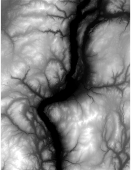
Images from a sample analysis are also provided for each step described in the tutorial. In the sample analysis, the Carp River watershed in Ottawa, Ontario is delineated, and a wetness index is generated for the watershed region. A DEM of the Ottawa-Gatineau region, with 50m cell size, was used for the sample analysis.
Figure 1: A 50m DEM for the Ottawa-Gatineau region that was used in sample analysis.
Setting Up Your Workplace
1. In QGIS, open the DEM using the 'Add Raster Layer' button in the 'Manage Layers' toolbar.
2. Once the DEM is loaded in QGIS, create a new GRASS mapset with an appropriate projection and workplace extent.
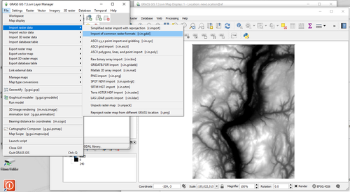
3. Using r.in.gdal.qgis, import the DEM into the new mapset.
Generating Watershed Boundaries:
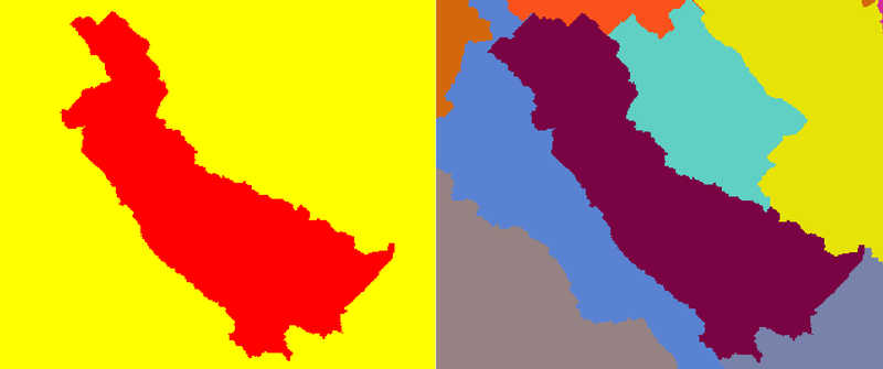
There are two available modules in GRASS that allow watershed delineation: r.watershed and r.water.outlet. Although these modules produce similar output, they delineate watersheds in two different ways.
r.watershed
- This method is designed for analysis in which the delineation of all watersheds over a specified size is required.
- If a watershed with a specific outlet point is required, use the r.water.outlet module.
To delineate watersheds in r.watershed:
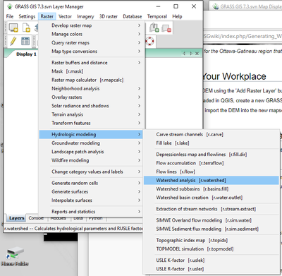
1. Open the r.watershed module.
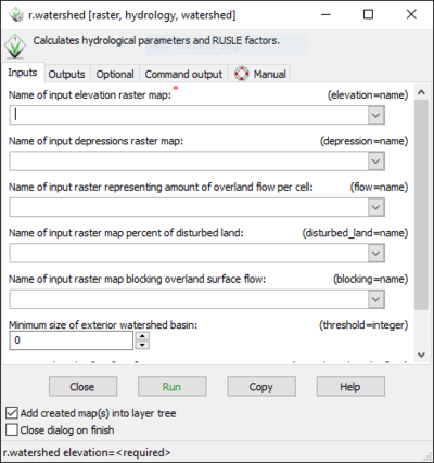
2. Select the DEM as the input map.
3. Select a proper input value. The input value (or threshold in the command line) refers to the minimum size in image pixels a watershed must contain to be delineated.
4. Specify a name for 'Output Map: Unique label for each watershed basin'.
Alternatively, this can be done in the command line:
- r.watershed elevation=DEM threshold=# basin=Watersheds
- This watershed output image will delineate all watersheds that exist within the DEM, given the threshold parameter that was specified.
- Each watershed in the image is assigned a unique pixel value.
Watershed Masks:
Since this method produces a watershed map consisting of numerous watersheds, if analysis on a particular watershed is required, a watershed mask will also be required.
A watershed mask can be produced in command line based on:
- r.mapcalc WatershedMask=if (Watersheds==’unique watershed label')
In the mask, areas within the watershed are assigned a value of 1, and all other areas are assigned a value of 0.
r.water.outlet
- Unlike r.watershed, this method will delineate a watershed based on the coordinates of its outlet point.
- This allows practitioners to customize the scale of output watersheds based on their research needs, without having to tamper with a threshold parameter.
To delineate watersheds in r.water.outlet:
1. Open the r.watershed module.
2. Select the DEM as the input map.
3. Specify a name for 'Output Map: Drainage Direction'.
- The output image quantifies the drainage direction of cells throughout the DEM.
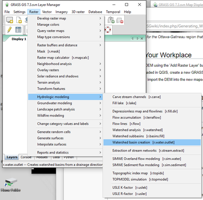
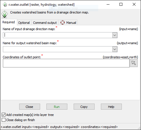
4. Open the r.water.outlet module.
5. Select the Drainage Direction map as 'Name of Input Raster Map'.
6. Specify the easting and northing of the watershed outlet point in 'The Map E Grid Coordinates' and 'The Map N Grid Coordinates'.
7. Specify a name for "Name of Raster Map to Contain Results'.
Alternatively, this can be done in command line based on:
- r.watershed elevation=DEM drainage=DrainageDirection
- r.water.outlet drainage=DrainageDirection basin=Watersheds easting=x northing=y
- The watershed output image will only include the watershed for which the outlet point was specified.
- The watershed output image is essentially a mask of the watershed.
Figure 2: Left: The watershed boundaries generated in r.water.outlet, using x,y coordinates obtained from a topographic map.
Right: The watershed boundaries generated in r.watersheds, using a threshold parameter of 10000.
Generating Wetness Indices:
Slope
This section will explain the steps involved in generating and preparing a slope image for the wetness index calculation.
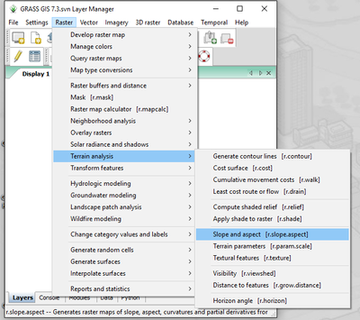
To generate a slope map in r.slope.aspect:
1. Open the r.slope.aspect.slope module.
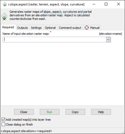
2. Select the DEM for ‘Name of Elevation Raster Map’.
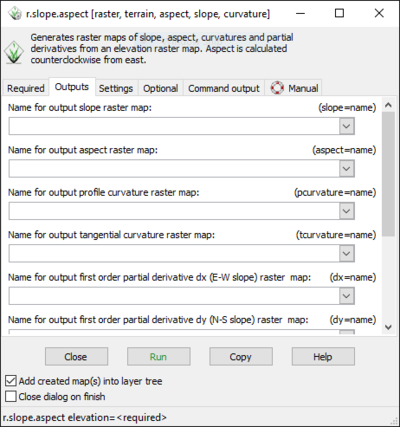
3. Specify a name for ‘Name for Output Slope Raster Map’.
Alternatively, this can be done in command line based on:
- r.slope.aspect elevation=DEM slope=Slope format=degrees
- The slope output image reports the slopes of the DEM landscape in degrees or percent slope, according to the user's choice.
- The slope image will commonly contain regions where slope equals zero.
- Since slope appears in the denominator of the wetness index equation, zero slope areas will result in undetermined (null) regions in the output wetness index maps.
Eliminating Zero Slope Areas in Slope Maps:
To avoid null values in wetness index images, zero slope areas in output slope images should be assigned a value of 0.0001 (or any other very small value).
To eliminate zero slope areas from slope maps:
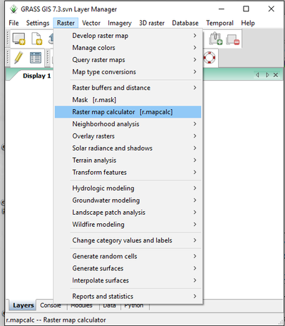
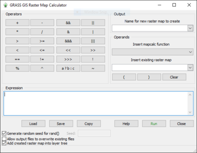
1. Open the r.mapcalculator module.
2. Select the output slope map as ‘A’.
3. Enter ‘A+0.0001’ as the ‘Formula’.
4. Specify a name for ‘Name for Output Raster Map’.
Alternatively, this can be done in command line based on [r.mapcalc Slope_NoZeros = Slope + 0.0001]
- This will replace zero slope values with slopes of 0.0001.
- The increase in slope in all other areas is negligible.
Upslope Contributing Area:
This section will explain the steps involved in generating and preparing an upslope contributing area image for the wetness index calculation.
To generate a flow accumulation map in r.watershed:
1. Open the r.watershed module.
2. Select the DEM as the input map.
3. Specify a name for 'Output Map: Number of Cells that Drain through Each Cell'.
Alternatively, this can be done in command line based on :
- r.watershed elevation=DEM accumulation=AccumFlow
- The output image quantifies the number of cells that drain through each cell or, in other words, the number of cells that are upslope from a given cell.
Since flow accumulation represents the number of upslope cells relative to a given cell, to obtain upslope contributing area, multiply flow accumulation by the area of cells in the image.
To generate an upslope contributing area map:
1. Open the r.mapcalculator module.
2. Select the flow accumulation image as ‘A’.
3. Enter ‘A * cell area’ as the ‘Formula’.
4. Specify a name for ‘Name for Output Raster Map’.
Alternatively, this can be done in command line based on [r.mapcalc UpslopeContributingArea = FlowAccumulation * ‘cell area’]
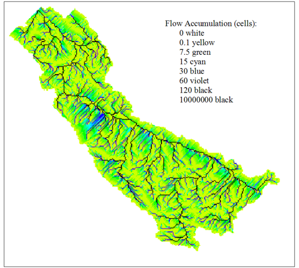
Figure 4: The output accumulated flow image and the user-defined color rules that were used to display the image.
Although the upslope contributing area is used to calculate wetness index, accumulated flow is illustrated in Figure 4 due to a time constraint. However, due to the nature of the upslope contributing area, the two images appear exactly the same.
Wetness Index:
Wetness index is calculated based on [WetnessIndex=ln(A/tan(B))] where A represents the upslope contributing area and B represents slope.
To generate a wetness index map:
1. Open the r.mapcalculator module.
2. Select the upslope contributing area image as ‘A’.
3. Select the slope image as ‘B’.
4. Enter ‘log(A/tan(B), 2.718282)’ as the ‘Formula’.
4. Specify a name for ‘Name for Output Raster Map’.
Alternatively, this can be done in command line based on:
- r.mapcalc WetnessIndex = log(UpslopeContArea/tan(Slope), 2.718282)
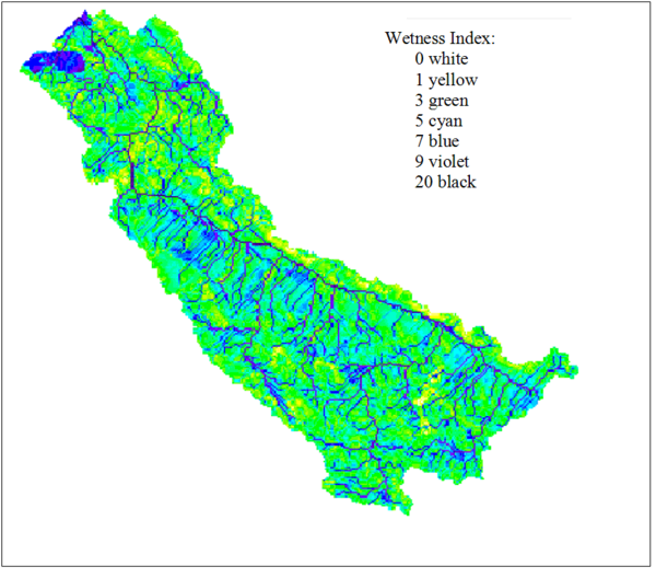
Figure 5: The output wetness index image and the user-defined color rules that were used to display the image.
Standardizing Wetness Index Maps:
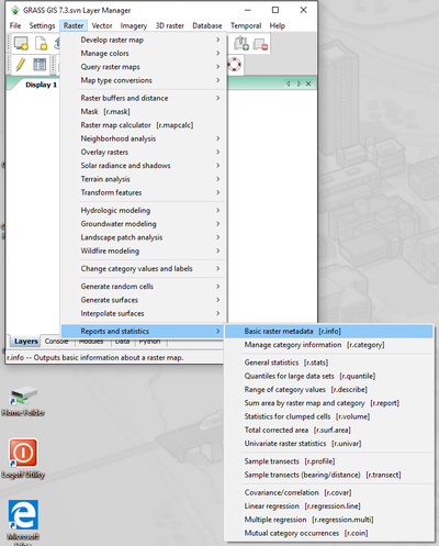
A common approach when comparing wetness indices is to standardize values between 0-1. If output wetness index images are going to be compared with other indices, standardize index values using r.mapcalc and r.info.
Standardizing images can be done in command line based on [r.mapcalc StandardizedImage= ((Image – ImageMin)/(ImageMax – ImageMin))].
Displaying Maps:
Given the extremely large flow values in creeks, streams, and tributaries within the watershed, flow accumulation and upslope contributing area images are often hard to interpret without user-defined color rules. Slope and wetness index images also required user-defined color rules for proper visual display.
To display images based on user-defined color rules:
1. Generate distributions for an image using the r.stats –c module in GRASS or the Histogram function in QGIS.
2. Based on the distribution and your research needs, determine suitable color breaks for displaying the image.
3. Create a text file (.txt) containing the color rules for the image.
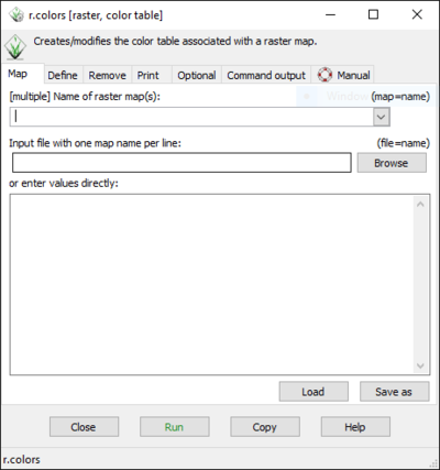
Refer to r.colors for syntax of color rules.
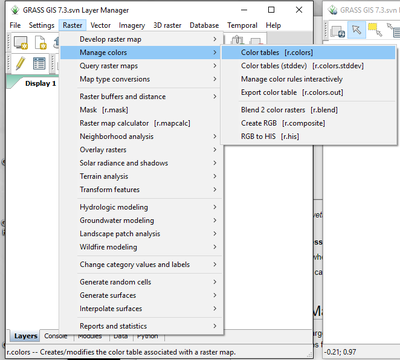
4. Open the r.colors module.
5. Select the image in ‘Name of Input Raster Map’.
6. Specify the full path to user-defined color rules text file in the ‘Path to Rules File’ browser.
Alternatively, this can be done in command line based on:
- r.colors map=FlowAccum rules=‘FullPathToColorRules’
DEM Filtering:
So far, all sample analysis images that are illustrated were generated from an unfiltered DEM. However, in order to achieve a specific level of detail in final wetness index images, filtering the DEM prior to generating the slope and flow accumulation maps may be required. Filtering can also reduce errors in future output maps that are caused by the DEM, or how the DEM was created. The DEM should be the only image that is filtered throughout the analysis. This ensures that all output images are derivatives of a specific elevation model. However, filtering final output maps for visual display is acceptable.
To apply a filter to a DEM:
1. Create a filter file which contains the filter you have chosen.
* In the sample analysis, the filter file contained a single 5x5 average filter; however, multiple filters can be included in one filter file.
* Refer to r.mfilter for the syntax of filter files.
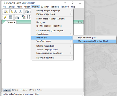
2. Open the r.mfilter module.
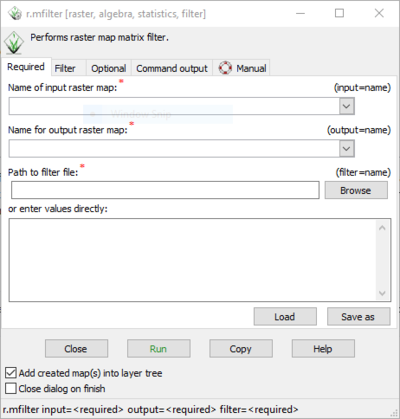
3. Select the DEM in ‘Name of Input Raster Map’.
4. Specify a name for ‘Name of Output Raster Map’.
5. Specify the full path and name of filter file in ‘Name of Filter File’.
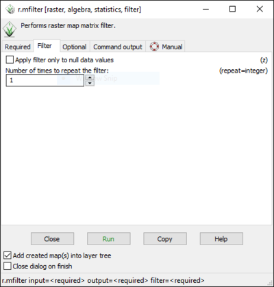
6. Specify the number of times to repeat the filter.
Alternatively, this can be done in command line based on [r.mfilter input=DEM output=DEM_filtered filter= ‘path to filter file’ repeat= ‘number of repeats’].
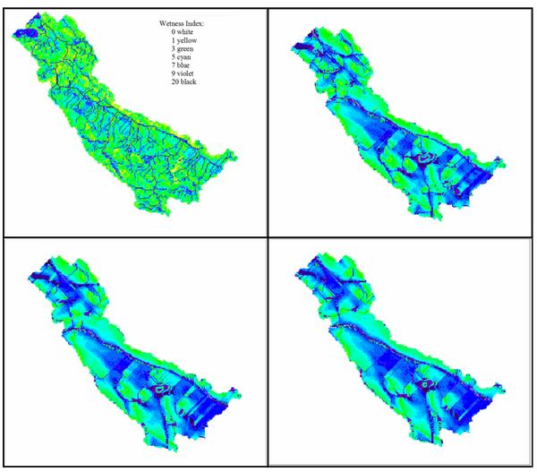
In the sample analysis, a total of four wetness indices were generated for the Carp watershed. All indices were generated using the methodologies described in this tutorial. Each was generated from a DEM that was filtered by a 5x5 average filter a varying number of times. The DEMs were filtered 0 times, 5 times, 10 times and 15 times prior to generating wetness index images. Screenshots of each wetness index are provided to allow an investigation into changes in wetness index that result from changes in DEM filtering processes.
Although these screenshots will convey the general effects of DEM filtering, trial and error will likely be required to find the proper series and types of filters for your research needs.
Figure 6: Wetness indices that were generated from a differently filtered DEM.
[Top Left: Unfiltered, Top Right: 5x5 filter x5 times, Bottom Left: 5x5 filter x10 times, Bottom Right: 5x5 filter x15 times]
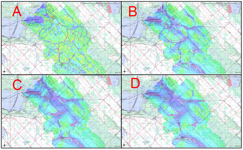
Figure 7: Wetness indices generated from differently filtered DEMs, superimposed on topographic maps during verification.
[A: Unfiltered, B: 5x5 filter x5 times, C: 5x5 filter x10 times, D: 5x5 filter x15 times]
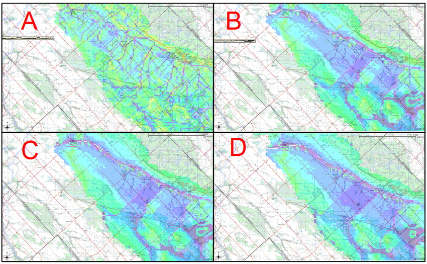
Figure 8: Wetness indices generated from differently filtered DEMs, superimposed on topographic maps during verification.
[A: Unfiltered, B: 5x5 filter x5 times, C: 5x5 filter x10 times, D: 5x5 filter x15 times]
Verifying Outputs:
Verifying Watershed Boundaries:
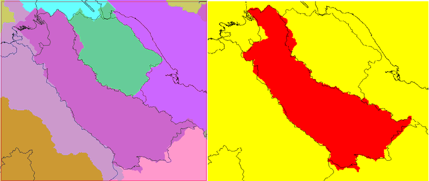
To assess the accuracies of the watershed boundary outputs, obtain digital maps (either raster or vector) of verified watershed boundaries from local conservation authorities. By superimposing the verified watersheds over the watershed outputs, the accuracy of watershed outputs can be visually evaluated. Note that, in Figure 9, the watershed delineated by r.water.color is more accurate that that delineated by r.watershed. This is likely due to an improper threshold parameter in r.watershed.
Figure 9: The two watershed outputs (Left: r.watershed, Right: r.water.outlet) and the watershed vector file, published by Ministry of Natural Resources.
Verifying Wetness Index:
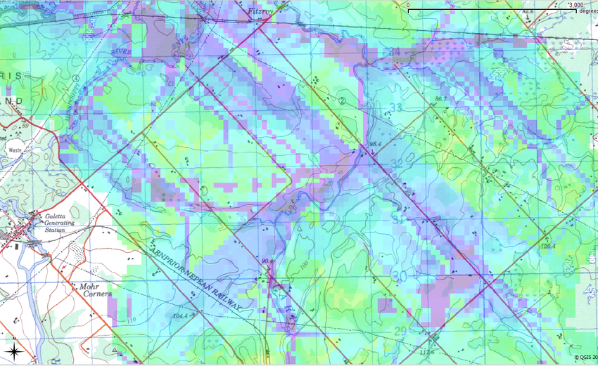
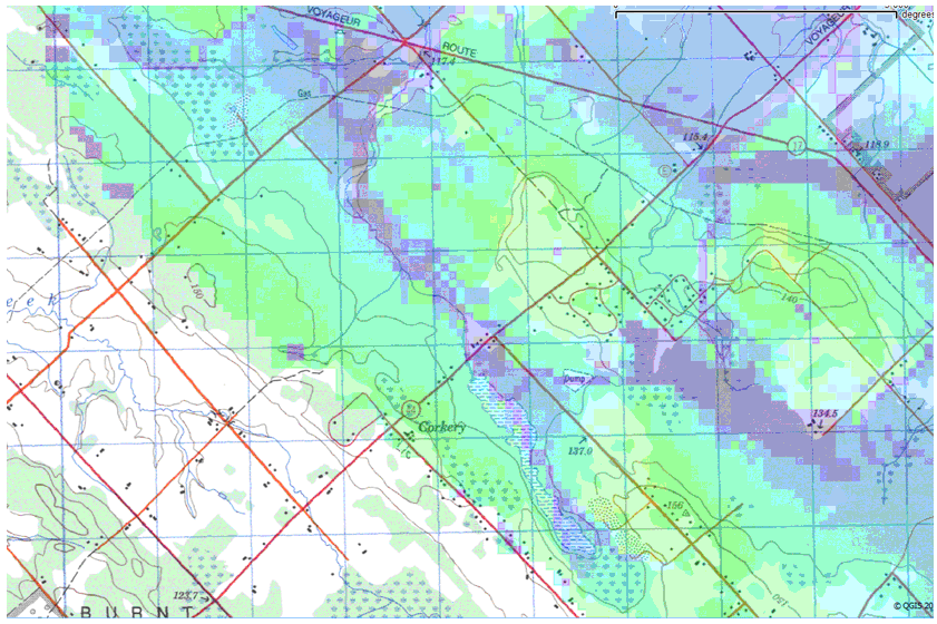
If digital topographic maps are available in your area, they can provide a good means of evaluating the potential accuracies of your output wetness index images. Superimpose the wetness index image (with the transparency of ~60%) over the topographic map. Based on the visual comparison between the two images, the accuracy of the wetness index can be evaluated. For example, if the majority of creeks, streams, and swampy areas on the topographic map are shown to be ‘wet’ areas on the wetness index, this would suggest a certain level of accuracy. On the other hand, if the majority of creeks, streams, and swampy areas on the topographic map are shown to be ‘dry’ areas on the wetness index, the index is likely inaccurate.
Figure 10: A screenshot during wetness index (from 5x5 average filtered DEM x5times) verification, in the northern region of the Carp watershed.
Figure 11: A screenshot during wetness index (from 5x5 average filtered DEM x5times) verification, in the southern region of the Carp watershed.
Additional:
For a practical and fully visual experience of working with QGIS and GRASS GIS in relation to the delineation of watersheds please see this two-part video from YouTube to further knowledge:
