Hydrological Analysis Using Whitebox Geospatial Analysis Tools

Purpose

The purpose of this tutorial is to guide the Quantum GIS (QGIS) user through the steps necessary to create a slope analysis model workflow using the Processing Toolbox. The user will also learn the basics surrounding the creation of slope, hillshade and aspect maps. The user will also then learn how to export the model as a Python script as well as preform geoprocessing tasks using the QGIS Raster Calculator. This tutorial is designed for a beginner GIS user who has experience with previous GIS software packages however no experience with QGIS.

Introduction

QGIS is a free open source geographical information system application that has geographical viewing, editing and analyzing capabilities. Within QGIS are tools called "Plug-ins". Plug-ins are essentially developed geoprocessing features made by the QGIS developers as well as independent users who would like to expand and contribute to the functionality of the software. One particular plug-in extension found in QGIS is the Processing toolbox extension. The Processing toolbox extension is similar to the features that are found in ArcMap’s ModelBuilder. Processing is an efficient application that is capable of creating, editing and managing geographical models. The user is able to connect together workflow diagrams that involve a series of geoprocessing algorithms. For the purposes of this tutorial, a workflow will be created using geographical data of Carp, Ontario in order to create a digital elevation model (DEM). This will then be used to create the slope, hillshade and aspect maps.

This tutorial was also done as a partial requirement of Carleton University's Advanced Topics in Geographic Information Systems 4008 course.

Data

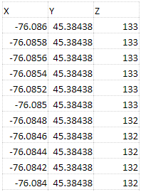
In this tutorial the only necessary layer is a Digital Elevation Model (DEM) file of your area of interest. In this tutorial we are focusing on Calabogie, ON. It is recommended that you use tthis same dataset for following along. It can be acquired and downloaded here. A sample of this data is shown bellow.

For the event that the dropbox link has become inactive the process of obtaining this data is described below to make this tutorial relevant for longer. Access the Government of Canada Geospatial Data Extraction Application here.

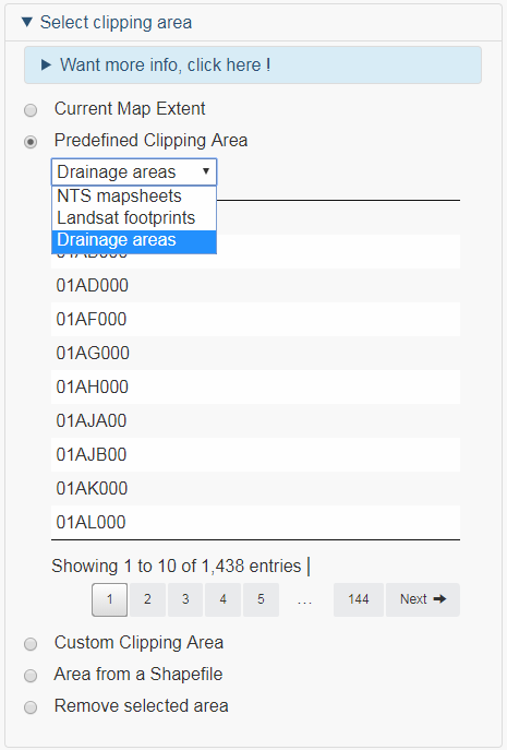
In the “Select Clipping Area” bar enter change the selection to "Predefined Clipping Area" and then select "Drainage areas" from the drop down list that appears.

This produces a long list of sequential drainage area names. Search through the names until you find "02KE000" and select it. I found this on the 17th page of drainage area names.

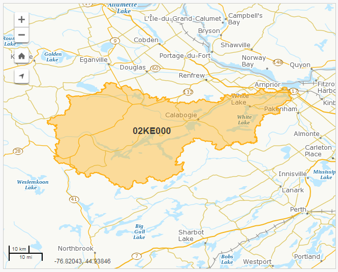
The map extent on the right side of the web page should now match the image below.

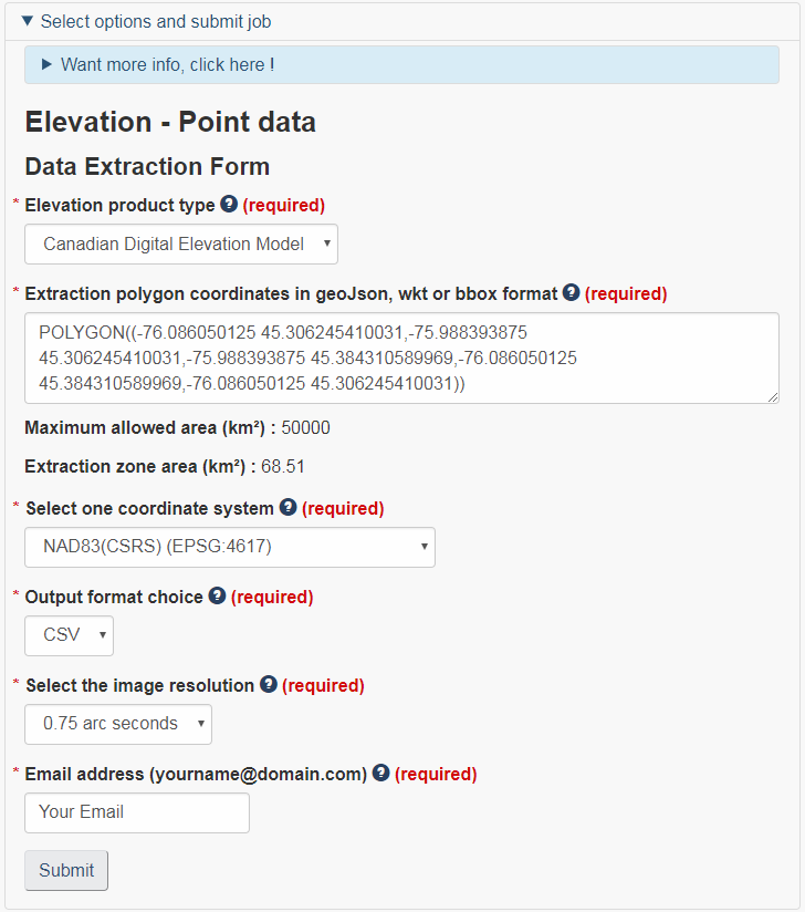
Next access the bar called “Select clipping area” and select “Current Map Extent”. Under “Select Data to be extracted” Select “Elevation – Point data”. Under “Select options and submit job” fill all of the required boxes so that it matches the figure below. Make sure to enter the email address that you would link to have the file sent to in the “Email Address” field.

An email will be sent to the entered email address shortly which contains a URL for the direct download of the data.

If neither of these options are available, since this tutorial starts with a basic csv file it can be run with any other point elevation csv file.

Acquiring QGIS 2.18.13

QGIS version: 2.18.13 (The current long-term release version of QGIS as of October20th 2017 is QGIS 2.18.13 and this was the version used for this tutorial. A list of the download links for all of the versions of QGIS can be found here.

Getting Started

Launching QGIS 2.18.13

When the installation process has finished, an icon should appear on your desktop similar to the one shown below.

Double-click on that icon and QGIS 2.18.13 will display on your screen.

Setting Project Coordinate Reference System (CRS)

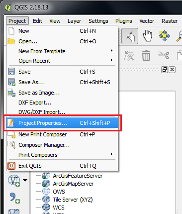
Following the launch of QGIS 2.18.13, navigate to the top menu bar, select Project, Project Properties, then CRS on the left column of the popup window.

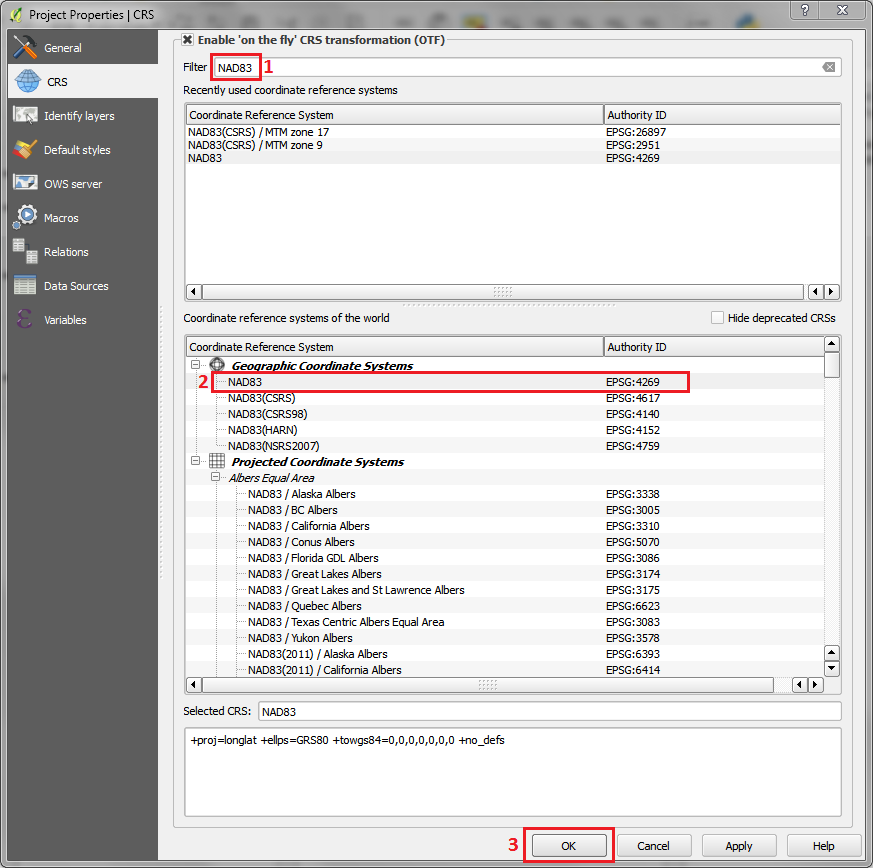
Make sure that Enable 'on the fly' CRS transformation is checked. Once enabled, filter search NAD83 (1) and select NAD83 under the Geographic Coordinate Systems (2). When finished select OK (3).

Adding Point Data

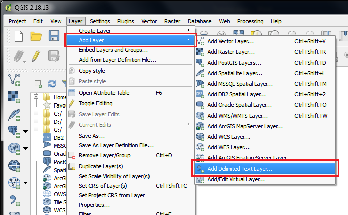
Adding the Carp elevation data or your desired .csv data requires navigating to the menu bar, select Layer and Add Layer, Add Delimited Text Layer....

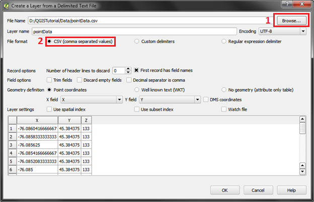
In the popup window browse for the .csv file that holds the elevation point data. Select CSV (comma separated values) for the file type. The rest of the options should default to the correct settings, but if the popup does not match the figure below make sure that you correct these differences.

Next you will be asked to choose the projection that the data has. As before filter search NAD83 (1) and select NAD83 under the Geographic Coordinate Systems (2). When finished select OK (3).

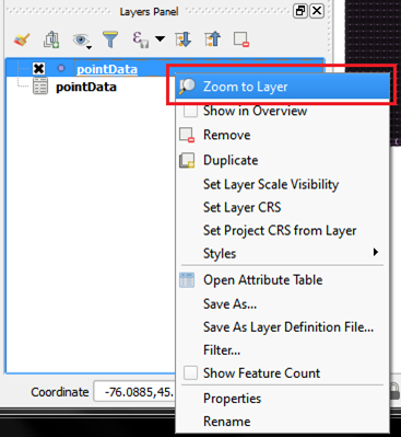
You should now be able to see your point data in the layers panel but your map view will not be focused on this data. Right click on the point data entry in the layers panel and select Zoom to layer.

Converting Point Data to a Shapefile

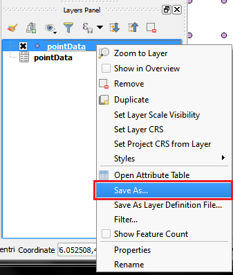
Next we will save this CSV file as a Shapfile to allow for more analysis to be done with it. Right click on the point data entry in the layers panel once again and select Save As…

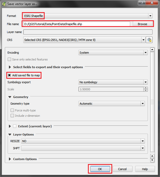
In the popup that appears set the format to ESRI Shapefile, set the file name and directory and ensure that the checkbox beside Add saved file to map is filled. Select OK once this is done.

You should now be ready for analysis.

Conclusion

In conclusion, this tutorial was aimed to give the user the skills to create workflows using the QGIS Processing Toolbox while also creating a workshop for slope and terrain analysis. This tutorial also gives the user the very basic introduction into the GIS world of Python scripting as well. The Python scripts that were exported can be slightly edited to preform the same geoprocessing tasks but with different parameters if necessary.

Resource Links

QGIS version 2.18 Documentation

GDAL - Geospatial Data Abstraction Library

Aspect - GIS Dictionary

Hillshade - GIS Dictionary

Interpolation - GIS Dictionary

Slope - GIS Dictionary

Python - Learn Python the Hard Way

Notepad++ Homepage

References

Crosetto, M., Tarantola, S., & Saltelli, A. (2000). Sensitivity and uncertainty analysis in spatial modelling based on GIS. Agriculture, Ecosystems and Environment, 81(1), 71-79. doi:10.1016/S0167-8809(00)00169-9

Hutchinson, M.F., 1998. Interpolation of Rainfall Data with Thin Plate Smoothing Splines – Part II: Analysis of Topographic Dependence. Journal of Geographic Information and Decision Analysis, vol.2, no. 2, pp. 152-167, 1998.

R.E. Crochiere and L.R. Rabiner. (1983). Multirate Digital Signal Processing. Englewood Cliffs, NJ: Prentice–Hall.