Hydrological Analysis Using Whitebox Geospatial Analysis Tools

Purpose

The purpose of this tutorial is to guide the user through an exploration of hydrology tools through the process of analyzing the hydrology of an area. This tutorial uses the opensource software Whitebox Geospatial Analyst Tools and explores some of the most useful of the hydrology tools included in it. The intent of this tutorial is for the user to understand the process underwent, an to be able to build off of it for their specific hydrology needs.

This tutorial assumes that the user has some experience with GIS software.

Introduction

This tutorial uses Whitebox 3.4.0, an open source GIS software that was developed within the In the Center for Hydrogeomatics in Guelph University. As a result this software package has a heavy focus on hydrological analysis. For this reason Whitebox was chosen for this tutorial on hydrological analysis. The area of focus in this tutorial is Calabogie Ontario. This location was chosen because the Calabogie peak adds some relief to the area, and the author knew it well enough to tell if there were any errors that occurred during the process.

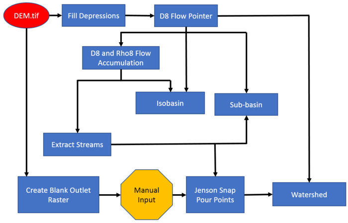
This tutorial uses a single input, a Digital Elevation model, and produces a multitude of outputs from it, adding information that could be used for future analysis. The process that will be undergone in this tutorial is displayed in the image below. To understand the context of each tool used in this tutorial please refer back to this image as needed.

Data Acquisition

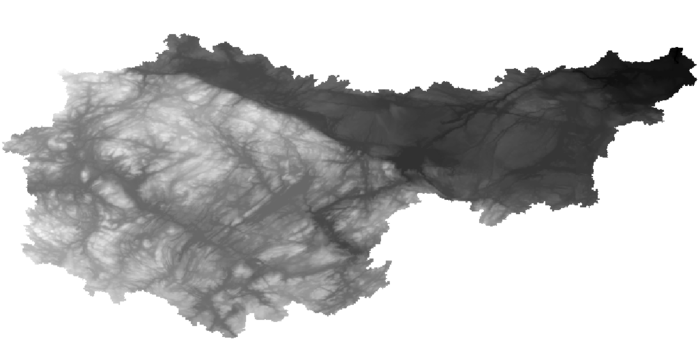
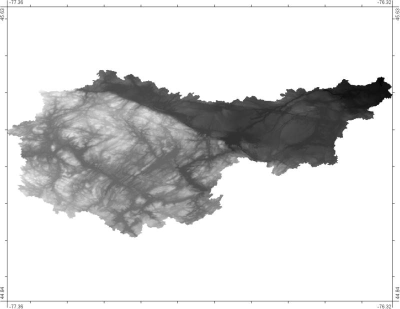
In this tutorial the only necessary layer is a Digital Elevation Model (DEM) file of your area of interest. In this tutorial we are focusing on Calabogie, ON. It is recommended that you use tthis same dataset for following along. It can be acquired and downloaded here. A sample of this data is shown bellow.

For the event that the dropbox link has become inactive the process of obtaining this data is described below to make this tutorial relevant for longer. Access the Government of Canada Geospatial Data Extraction Application here.

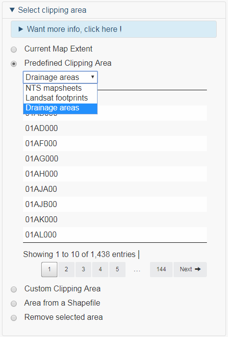
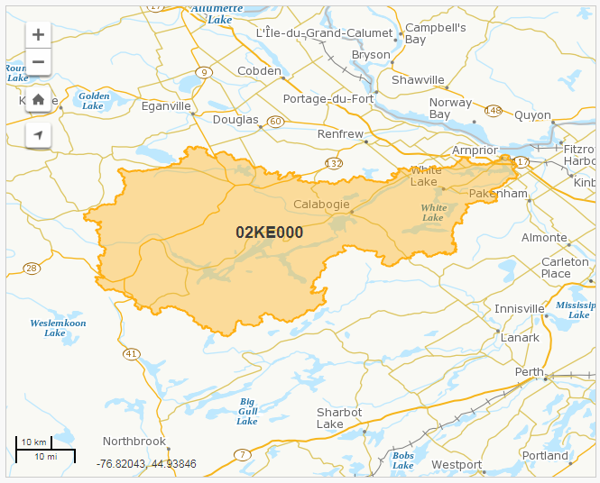
In the “Select Clipping Area” bar enter change the selection to "Predefined Clipping Area" and then select "Drainage areas" from the drop down list that appears.

This produces a long list of sequential drainage area names. Search through the names until you find "02KE000" and select it. I found this on the 17th page of drainage area names.

The map extent on the right side of the web page should now match the image below.

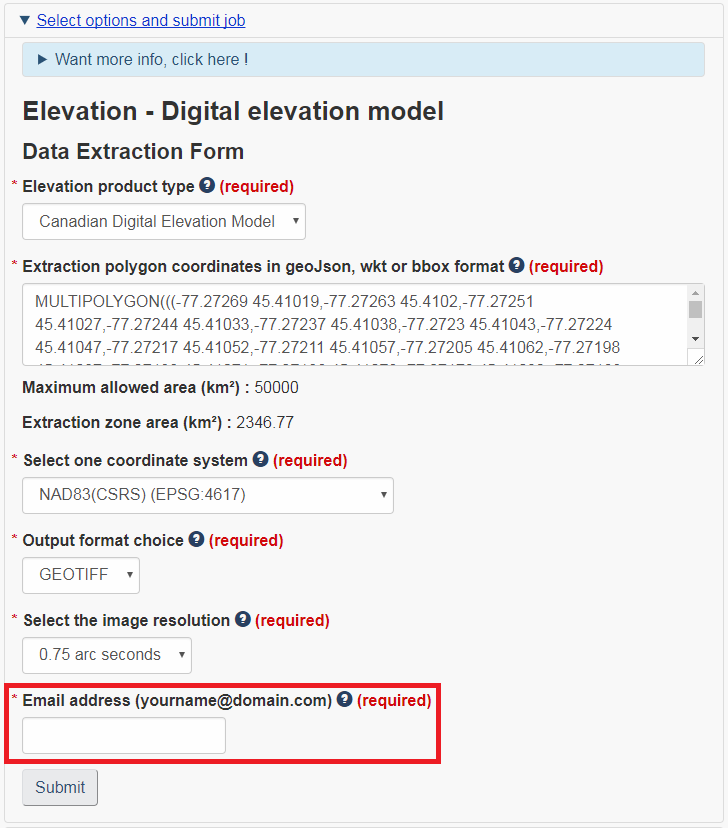
Under “Select Data to be extracted” Select “Elevation – Digital elevation model”. Under “Select options and submit job” fill all of the required boxes so that it matches the figure below. Make sure to enter the email address that you would like to have the file sent to in the “Email Address” field.

An email will be sent to the entered email address shortly which contains a URL for the direct download of the data.

If neither of these options are available, any DEM in a tiff format can be used.

Acquiring and Installing Whitebox 3.4.0

Whitebox version: 3.4.0 (The current version of Whitebox as of 2017 is 3.4.0 and this was the version used for this tutorial. A list of the download links for Windows, Mac and Linux platforms can be found here.)

After the correct .zip file has been downloaded and extracted to your directory of choice the installation process is complete.

It is important that your machine has version 8 or higher of the Java SE Runtime Environment before trying to run Whitebox. This can be acquired here

Getting Started

Launching Whitebox 3.4.0

After the file has been extracted the contents should look similar to the image below

Double click on the "WhiteboxGIS.jar" file in order to launch the program.

Note: If you are running Windows 10 on your computer you may need to double click on the "Whitebox.bat" file to launch it instead.

Setting up a working Directory

For this Tutorial I created a working directory before starting any analysis processes. This step is not necessary, though it will aid in the organization of this project. Create a folder called "WhiteboxTutorial", or something similar. Within this folder create one folder called "Data", and another called "DataProducts"

The final product will look like the image below.

Place the DEM.tif data file into the "Data" folder. All files created from the DEM file will be placed in the "DataProducts" folder. i.e. all files output by Whitebox tools while going through this tutorial. Also, project files will be saved directly within the "WhiteboxTutorial" folder itself.

Adding Elevation Data and Saving the Map Project

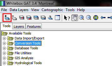
To add the elevation data to the project select the icon in the top left of the Whitebox window, highlighted in red in the image below. (or use the hotkey Ctrl + L)

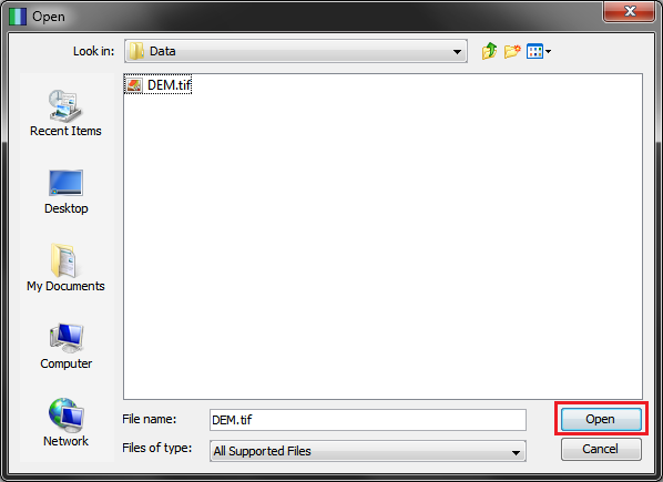
A popup window will then appear. In this window navigate to the location of the Calabogie DEM data file and select open.

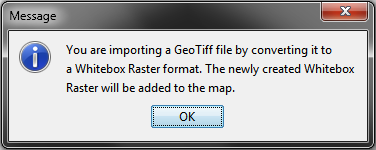
You will likely recive a popup message like the one below. Select okay to add your data to the map.

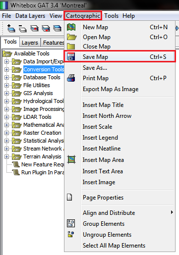
To save your project select "Save Map" under the "Cartography" tab. (or use the hotkey Ctrl + S)

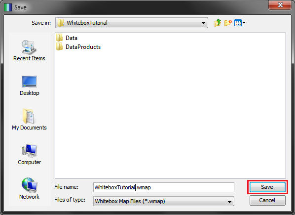
In the pop up window that appears navigate to the location that you would like to save the project and select "Save".

You should now be ready for analysis.

Hydrological Analysis

DEM Pre-Processing

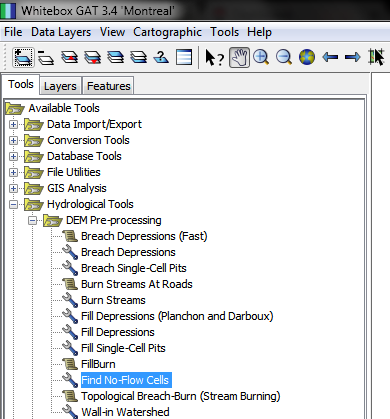
Pre-processing is an important first step in any hydrological analysis as this process identifies and corrects all features within the DEM that may disrupt the flow analysis. Since all products are derived from the DEM it is important to make these corrections at the begging of the process to prevent these errors from carrying through into all of the hydrological outputs. All of the DEM Pre-Processing tools available in Whitebox can be found in the tools menu under the following directory: Tools> Hydrological Analysis> DEM Pre-Processing

The first tool used in this tutorial is "Find No-Flow Cells", found in the highlighted location in the image below. This was used to identiy if there were any problem areas, and how extensive they were.

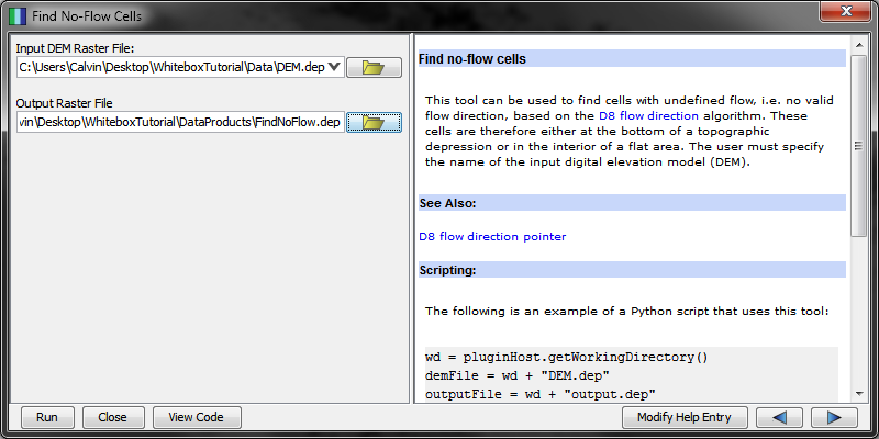
After double clicking the tool name in the tools list the dialogue box in the image bellow will appear. Set the Calabogie area DEM as the "Input DEM Raster File". Make sure that the "Output Raster File" will be saved within the DataProducts folder in the directory you set up and give it a name similar to "FindNoFlow.dep". After these inputs have been set click "Run" in the bottom left of the popup window.

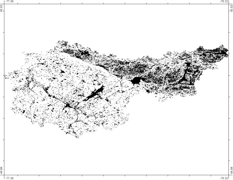
After the tool runs it will produce a file that looks like the one below. The black areas in this image are all of the problem areas identified that could cause problems for flow analysis. These areas tend to correspond with errors in the DEM if they are small, or basins in the landscape if they are large. The high amount of no flow areas identified using this tool means that a pre-processing correction tool will be necessary.

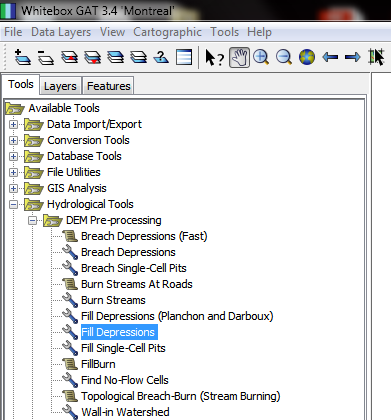
In this tutorial the "Fill Depressions" tool is used to correct the no flow areas. This was chosen because it is much more computationaly efficient than any of the breach tools, finishing much quicker. This tool if found in the location below.

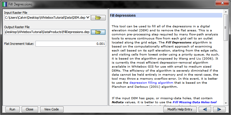
The dialog box that appears for this tool is shown below. The input file should be set to the original Calabogie DEM, and the output should be set to the DataProducts folder and named something similar to "FillDepressions.dep". The "flat increment value" is the step value added to cells within a flat area in order to ensure that they have a slight slope instead of remaining flat. This was kept at the default value of "0.001".

The output of this tool is shown below. It does not appear very different to the original DEM, but will closer inspection differences within the areas identified in the Find No-Flow Cells output can be seen.

Flow Pointer

A flow pointer tool in Whitebox is a tool that identifies which area surrounding a cell is the lowest. The value of this cell is then assigned corresponding to the relative direction of this area. This information is not too useful on its own, but it is used as an input to many other hydrology tools because it denotes the direction that water will flow from each cell.

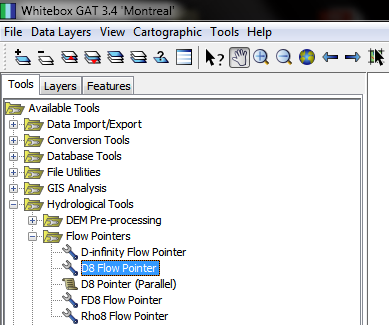
Whitebox has many different flow pointer tools that each use a different method to produce their results. In this tutorial "D8 Flow Pointer" was used because many of the tools in the "Watershed Tools" toolset will only work with the output from the D8 Flow Pointer as an input. This tool is found in the location shown below.

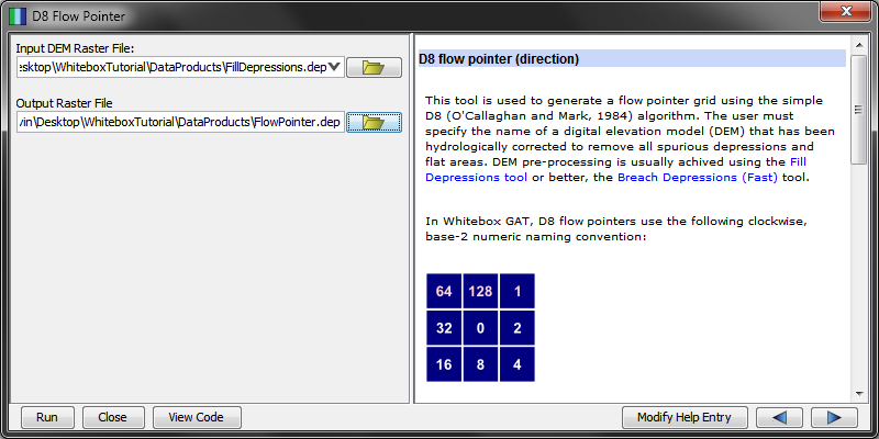
The dialog box for this too is shown below. The input DEM raster file should be set to the output from the Fill Depressions tool (FillDepressions.dep), and the output should be set to the DataProducts folder and named something similar to "FlowPointer.dep"

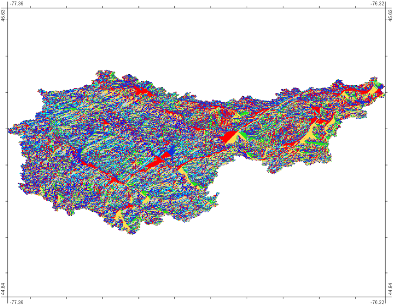
The output from this tool is displayed below. This image contained 8 colours corresponding to the 8 directions of flow. This image appears chaotic, but will be used in other tools to create more informative data products.

Flow Accumulation

Flow Accumulation tools analyze the magnitude of cells that pour into or through an area. This is useful on its own, allowing us to determine the relative flow through areas by comparing values of the output, and is also used as an input for many other analyses.

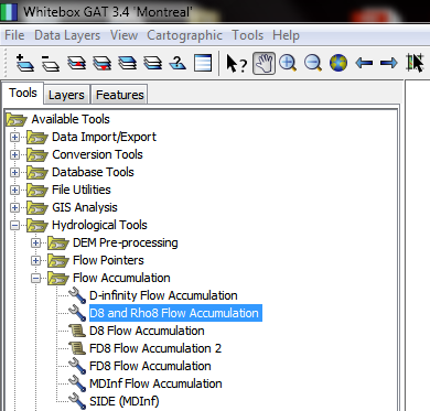
In this tutorial the "D8 and Rho8 Flow Accumulation" tool was used, as this was the one that corresponded to the D8 Flow Pointer output that was created with the previous tool. This tool is located in the location displayed below.

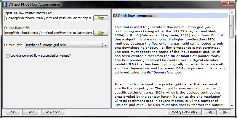
The dialog box for this tool is displayed below. The input D8 flow pointer raster file should be set to the output from the D8 flow pointer tool (FlowPointer.dep), and the output should be set to the DataProducts folder and named something similar to "FlowAccumulation.dep". In the example the "Output Type" was set to "number of upslope grid cells" so that a greater cell value in the output would correspond to a greater number of cells flowing through that cell. The "Log-transformed flow accumulation values?" box was left unchecked in this example, though checking this would help normalize the data for better display.

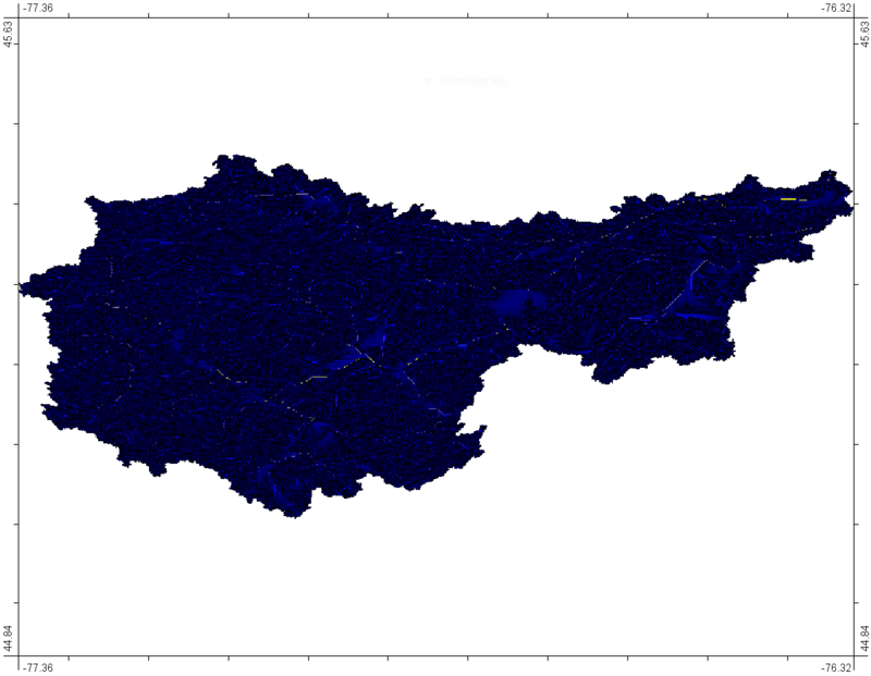
The output of this tool is displayed below. The brighter areas correspond to areas of higher accumulated flow. These areas of high flow correspond to the areas where more water gathers and flows together. A beter picture of the data can be gathered by zooming into the output in Whitebox.

Isobasin

The isobasin tool divides a study area into equally sized drainage areas (iso-basins) of a specified size.

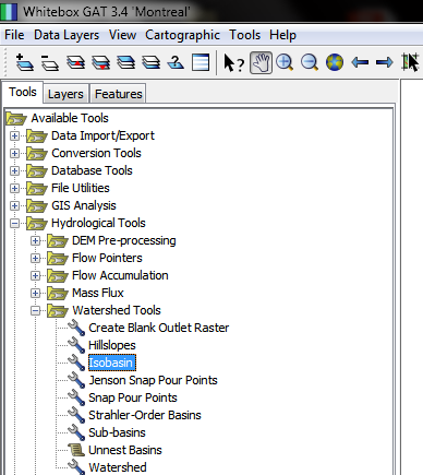
The location of this tool is displayed below.

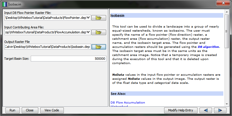
The dialog box for this tool is displayed below. The input D8 flow pointer raster file should be set to the output from the D8 flow pointer tool (FlowPointer.dep), and the input contributing area file sould be set to the output from the D8 and Rho8 Flow Accumulation tool (FlowAccumulation.dep). The output should be set to the DataProducts folder and named something similar to "Isobasin.dep". For this example the "Target Basin Size" was set to 500,000 cells. This value was found using trial an error to find an output that looked appropriate.

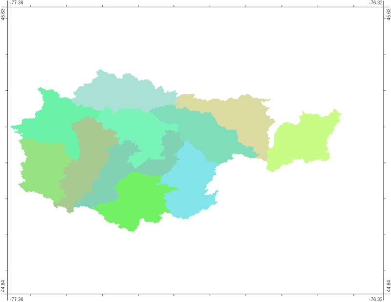
The output from this look is displayed below. It can be seen that the area has been broken down into 11 different basins of approximately equal size. It also appears that the basins do not fill the entire study area. This is likely because no more basins of a size of 500,000 cells could be fit into these areas. If the target basin size was set to a lower number these basins would conform to the study area more completely

Extract Streams

Sub-basins

Watershed Analysis

Pour Points

Watershed

Conclusion

In conclusion, this tutorial was aimed to give the user the skills to create workflows using the QGIS Processing Toolbox while also creating a workshop for slope and terrain analysis. This tutorial also gives the user the very basic introduction into the GIS world of Python scripting as well. The Python scripts that were exported can be slightly edited to preform the same geoprocessing tasks but with different parameters if necessary.

Resource Links

QGIS version 2.18 Documentation

GDAL - Geospatial Data Abstraction Library

Aspect - GIS Dictionary

Hillshade - GIS Dictionary

Interpolation - GIS Dictionary

Slope - GIS Dictionary

Python - Learn Python the Hard Way

Notepad++ Homepage

References

Crosetto, M., Tarantola, S., & Saltelli, A. (2000). Sensitivity and uncertainty analysis in spatial modelling based on GIS. Agriculture, Ecosystems and Environment, 81(1), 71-79. doi:10.1016/S0167-8809(00)00169-9

Hutchinson, M.F., 1998. Interpolation of Rainfall Data with Thin Plate Smoothing Splines – Part II: Analysis of Topographic Dependence. Journal of Geographic Information and Decision Analysis, vol.2, no. 2, pp. 152-167, 1998.

R.E. Crochiere and L.R. Rabiner. (1983). Multirate Digital Signal Processing. Englewood Cliffs, NJ: Prentice–Hall.