Difference between revisions of "Cost Path Analysis of Mars using SAGA"
| (82 intermediate revisions by the same user not shown) | |||
| Line 1: | Line 1: | ||
=Purpose= |
=Purpose= |
||
This tutorial will describe the detailed steps required to perform Cost Path Analysis using [http://www.saga-gis.org/en/index.html SAGA GIS], a free and open source software. |
|||
It will use SAGA’s Grid tools to perform terrain analysis and basic grid/raster processing using a digital terrain model (DTM) from the surface of Mars, as well as Shape tools for some vector dataset creation. |
|||
Finally, there will be an introduction to some tools and processes used in more advanced cost-path analysis. |
|||
=Objective= |
|||
This tutorial aims to provide step-by-step instructions for completing cost-path analysis within SAGA. |
This tutorial aims to provide step-by-step instructions for completing cost-path analysis within SAGA. |
||
The basic analysis will use tools from the following built-in libraries: Grid, Shape and Terrain Analysis. |
The basic analysis will use tools from the following built-in libraries: "Grid", "Shape" and "Terrain Analysis". |
||
A more advanced analysis will further explore tools within the Grid library. |
A more advanced analysis will further explore tools within the Grid library. |
||
By the end, this tutorial will have shown you how to use SAGA’s built-in tools to perform a cost-path analysis using a Mars DTM and be exposed to more advanced techniques to enhance the basic cost-path analysis. |
By the end, this tutorial will have shown you how to use SAGA’s built-in tools to perform a cost-path analysis using a Mars DTM and be exposed to more advanced techniques to enhance the basic cost-path analysis. |
||
| Line 14: | Line 9: | ||
=Introduction= |
=Introduction= |
||
== SAGA == |
=== SAGA === |
||
SAGA is an open source program for GIS that has a lot of capability in geoscientific analysis and has been designed for effective implementation of spatial algorithms. It features an extensive suite of tools covering raster data (called Grid data within SAGA) and operations, imagery processing, vector processing as well as some ecological and geomorphological simulations, to name a few. |
SAGA is an open source program for GIS that has a lot of capability in geoscientific analysis and has been designed for effective implementation of spatial algorithms. It features an extensive suite of tools covering raster data (called Grid data within SAGA) and operations, imagery processing, vector processing as well as some ecological and geomorphological simulations, to name a few. |
||
More information can be found at their [http://www.saga-gis.org/en/index.html homepage], and the latest version of |
More information can be found at their [http://www.saga-gis.org/en/index.html homepage], and the latest version of the software can be [https://sourceforge.net/projects/saga-gis/ downloaded from SourceForge.] This tutorial uses SAGA v6.4.0. |
||
To see more CUOSG tutorials that have used SAGA GIS, [https://gracilis.carleton.ca/CUOSGwiki/index.php?title=Special%3ASearch&search=SAGA&go=Go click here] |
|||
== Cost-Path Analysis == |
|||
=== Cost-Path Analysis === |
|||
(insert intro on CPA here, note least cost path we will use) |
|||
Cost-path Analysis is a GIS tool used for distance analysis and is primarily used for determining the most efficient route between two points. The strength of cost path analysis is its flexibility in modelling applications as it is only limited by what costs can be assigned to travel a distance. As a result, cost path analysis can be used in a variety of applications, and has been used to determine the best routes for power transmission lines, developing walking paths, determining ecological corridors for wildlife movement as well as [https://gracilis.carleton.ca/CUOSGwiki/index.php/Fire_spread_through_cost_path_analysis_in_QGIS_GRASS modelling fire spread] and flooding. |
|||
More details about cost path analysis can be found [https://www.gislounge.com/overview-least-cost-path-analysis/ here]. |
|||
=Background and Data= |
=Background and Data= |
||
This tutorial will explore Northeast Syrtis, which refers to the northeast |
This tutorial will explore the Northeast Syrtis region of Mars, which refers to the northeast area of [https://en.wikipedia.org/wiki/Syrtis_Major_quadrangle Syrtis Planum Major quadrangle], which is a candidate landing spot for the [https://mars.jpl.nasa.gov/mars2020/ Mars 2020 rover mission]. As part of the preparation for the mission, stereo images of the potential landing site were taken by NASA’s Mars Reconnaissance Orbiter. The images were then used to create a digital terrain model (DTM), with the primary objective of being used in the rover mission’s Entry, Descent and Landing (EDL) simulations. |
||
The DTM of NE Syrtis [https://astrogeology.usgs.gov/search/map/Mars/Mars2020/landing_site/B18_016575_1978_B17_016219_1978_20m_DTM (download here)] is made available by the [https://astrogeology.usgs.gov/ USGS Astrogeology Science Center]. |
The DTM of NE Syrtis [https://astrogeology.usgs.gov/search/map/Mars/Mars2020/landing_site/B18_016575_1978_B17_016219_1978_20m_DTM (download here)] is made available by the [https://astrogeology.usgs.gov/ USGS Astrogeology Science Center]. |
||
For our analysis, we will be using the DTM to determine |
For our analysis, we will be using the DTM as a base to determine a hypothetical path for the rover once it has landed. |
||
A crucial element to note in this analysis is the type of coordinate system required. |
|||
Any cost path analysis requires a projected coordinate system, which measures distance in units of distance (such as meters or feet), rather than a geographic coordinate system which uses angular units (degrees or radians). In this way, the analysis represents a cost associated with a consistent distance/area rather than angles, which vary in size as distance to the poles vary. |
|||
Since we are using data from another planet, special attention must be given to the coordinate system. Fortunately, the DTM used in this example comes projected in an appropriate coordinate system and is ready for our analysis. |
|||
=Methods= |
=Methods= |
||
=='''Basic Cost Path Analysis'''== |
|||
==='''Uploading Data into SAGA'''=== |
|||
The first step is to upload a DEM into Saga, because this program has very specific file formats that it can handle, a previous tutorial will show how this is done. It can be found within [http://gracilis.carleton.ca/CUOSGwiki/index.php/Exploring_Hydrological_Analyses_using_SAGA_GIS Exploring Hydrological Analyses]. |
|||
The first step of the process is to download the DTM. The DTM of NE Syrtis comes in a TIFF (.tif) file format, which is a common file type for raster data in geospatial analysis. |
|||
==='''Creating Points'''=== |
|||
Once the file is downloaded, open the SAGA software. Start with an empty startup project. |
|||
To import the DTM, go to “File >> Grid >> Load” and navigate to where you stored the DTM. Click Open. The file might take a little while to load. |
|||
To create points on a layer, go into Geoprocessing>>Shapes>>Points>>Create Point Grid, this will bring up a window. |
|||
Next, double click the file you just imported. A map should appear, and look like the image below. |
|||
[[Image:Map_with_DTM_imported.PNG|395px]] |
|||
[[File:create_point_grid.png]] |
|||
The presence of the scale bar with units in Kilometers indicates that we have a projection suitable projection. To check the details, navigate to the “Description” tab in the properties window, and check the Projection. It should say “EquirectangularMars”, with its parameters below. |
|||
[[Image:Projection_annoted.PNG|500px]] |
|||
Save it to where your files are, click okay and a new shape layer will be created within your data window, within that window right click on the "Point Grid" and go into edit and "add shape". |
|||
Now we’ll rename a few things to make the analysis process smoother. |
|||
First we’ll rename the Grid System, the first entry under “Grids” in the data tab (1. in photo below). Under the “Settings” tab in the Properties window, click to the right of the “Name” field. I chose to rename it “Syrtis Grid System”. |
|||
Next we’ll do the same for the DTM itself. Click on the DTM layer (2. in photo below), then repeat the above process. I named the DTM “Syrtis 20m DTM”. |
|||
[[Image:Named grid and system annot.PNG|560px]] |
|||
[[File:Point_grid_window.png]] |
|||
Now we’re ready to continue with the analysis. |
|||
==='''Creating Points'''=== |
|||
To perform our cost-path analysis, we need to create a starting point and ending point for our path. To do so we will need to create two new vector layers. |
|||
Using the action tool [[File:action_tool.png]], create points by selecting the location on the map, then right click and click edit selected shape, and apply the changes. To create multiple, right click and add shapes. |
|||
To create a vector layer, we’ll use the geoprocessing tools. Navigate to “Geoprocessing >> Shapes >> Construction >> Create new “Shapes layer”. Check that the Shape Type is Points, then change the name to “Rover_start”. Click Okay. |
|||
[[Image:Create point layer Rover start.PNG|550px]] |
|||
[[File:Points_on_Mars.png]] |
|||
Repeat the process to create the “Rover_end” layer. |
|||
==='''Kriging'''=== |
|||
Under the Data Tab in the Manager on the left, you should see the three elements we have so far. Double click each point shape to add it to the map. The map panel should look like the following. |
|||
[[Image:Map_with_point_shapes.PNG|300px]] |
|||
To be able to add the points to a grid layer, Ordinary Kriging will be done. For the uses of different Kriging methods the information can be found at [http://www.saga-gis.org/saga_module_doc/2.1.3/a2z.html Full Module Index] |
|||
by going into Geoprocessing>>Spatial and Geostatistics>>Kriging>>Without Variogram Fit>>Ordinary Kriging. |
|||
Next we need to create the points on our map. To do so, click on the layer you want to edit in the Maps tab. Right click, go to “Edit >> Add Shape”. From the top menu bar, click on the arrow pointer, called the “Action Tool”. |
|||
[[File:Ordinary_Kriging.png]] |
|||
[[Image:Add points action tool.PNG|550px]] |
|||
Next, left-click somewhere in the top half of the map; this will be our starting point. When you’re happy with the location, right-click and select “Edit Selection” and click “Yes” on the window that pops up. |
|||
This window should appear; add the point grid created in the "Points" section, also change target grid to "Grid System". Click okay and another window should appear. |
|||
Repeat for the end point, this time placing the point near the bottom of the map. You should now have two points on your map. |
|||
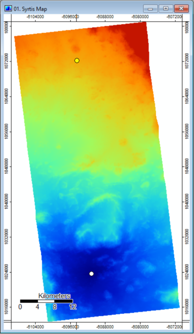
[[Image:Map_start_end_points.PNG|400px]] |
|||
We are now ready to move on to the Terrain Analysis portion of the analysis. |
|||
[[File:Kriging_Grid_selection.png]] |
|||
Select the appropriate grid system and select okay and an image should appear. |
|||
[[File:Kriged_image.png]] |
|||
==='''Terrain Analysis'''=== |
==='''Terrain Analysis'''=== |
||
This portion of the analysis turns our DTM into a set of derivative terrain products from which we will base our cost path analysis from. SAGA has a convenient tool that can calculate slope, aspect and curvature within a single window. |
|||
The terrain analysis within Saga has a simple method of selecting any surface that you would like to determine all within one window. By going into Terrain Analysis>>Morhpometry>>Slope, Aspect, Curvature. A window should appear that will give you available options of what processes can be done. |
|||
To create the terrain products, go to “Geoprocessing >> Terrain Analysis >> Morphometry >> Slope, Aspect, Curvature”. |
|||
- The Grid layer was selected, |
|||
The inputs are “Syrtis Grid System” for the grid system and “Syrtis 20m DTM” for the elevation. |
|||
To get our outputs, we need to select “<create>” on the following elements: “Slope”, “Aspect” and “Cross-Sectional Curvature”. |
|||
We will also change the units for both Slope and Aspect to degrees. |
|||
[[Image:slope_annot.PNG|800px]] |
|||
- The DEM elevation was Chosen, |
|||
- In the drop down tabs, create was selected beside Slope, Aspect, Cross sectional Curvature |
|||
When all the options have been correctly set, click Okay. The outputs can now be found in the Data tab of the Manager. Below is an image of the three outputs. |
|||
- In methods, a 9 parameter 2nd order polynomial was chosen, |
|||
[[Image:Slope_aspect_curve_output_side_by_side.PNG|800px]] |
|||
- Slope and Aspect units, where changed to Degrees |
|||
[[File:Slope_Aspect_Curvature.png]] |
|||
==='''Reclassify'''=== |
|||
We have created some terrain products, but they aren’t particularly meaningful for use in cost path analysis right away. We will be using the Slope layer as the basis of our analysis and we will reclassify some of the values to better represent the difficulty of crossing varied terrain. |
|||
The following three figures were produced by the Terrain Analysis tool. |
|||
To start reclassifying, navigate to “Geoprocessing >> Grid >> Values >> Reclassify Grid Values”. In the tool menu, select the following inputs: “Syrtis Grid System” for the grid system, “Slope” for the grid. |
|||
Next, we need to define the method for reclassifying the raster. Under Method, select “simple table”. |
|||
[[Image:reclass_tool.PNG|600px]] |
|||
[[File:Slopemars.png]] |
|||
On the next line below, click the three dots on the right-hand line of “Lookup Table”. This should open a new window. Add some lines and enter the values to look like the following photo. |
|||
Figure 1: Slope of Mars Terrain, indicating slope |
|||
[[Image:slope_reclassed_values.PNG|700px]] |
|||
When happy with the values, click Okay on the Lookup Table window, then Okay on the tool. Below is a photo of the reclassified slope layer. |
|||
[[File:Aspect1.png]] |
|||
[[Image:slope_map_reclassed.PNG|395px]] |
|||
Figure 2: Aspect of Mars Terrain, showing the location of the aspect |
|||
The values selected for reclassification were arbitrarily determined and will be sufficient for this process. However, determining appropriate cost values, as will be discussed later, is one of the most difficult elements of cost path analysis. |
|||
==='''Accumulation Cost'''=== |
|||
Now that we have created our terrain products and reclassified our slope data into something meaningful, we are ready to begin the cost-path analysis. |
|||
[[File:Cross-Sectional_Curvature1.png]] |
|||
The first step is to create an accumulation cost surface. Given a vector point (our destination point), this tool returns a surface that represents how “expensive” it is to travel away from the given input point. This will be the input for the final step of our least cost path analysis. |
|||
To create the accumulation cost surface, navigate to “Geoprocessing >> Grid >> Analysis >> Cost Analysis >> Accumulation Cost”. The inputs should be "Syrtis Grid System" for the grid system, "Slope_reclassified" for the local cost, and "Rover_end" as the destination point. Once this is done, click Okay. |
|||
Figure 3: Cross-Sectional Curvature of Mars Terrain |
|||
The output will show up on the “Data” tab labeled “Accumulated Cost”. Double click it to add it to the map. |
|||
Below is an image of the accumulation cost raster. It shows areas of low cost in blue (near the end point) and areas with increasing cost in red. |
|||
==='''Reclassify'''=== |
|||
[[Image:Accumulated_cost_with_points.PNG|395px]] |
|||
To reclassify the values to set range and remove empty cells, go into Geoprocessing>>Grid>>Values>>Reclassify Grid Values. |
|||
- Select the Grid system that needs to be reclassified. |
|||
Now we move on to complete the last step in our analysis. |
|||
- Select the Grid, the DEM mars is shown, same processes is done with Slope. |
|||
==='''Least Cost Path'''=== |
|||
- Choose the values that want to be reclassified. In this case 0 to 1. |
|||
To complete our analysis and see the final product, we will finally run the Least Cost Path analysis tool. |
|||
- No Data value of input can be selected here as well. |
|||
It can be found under “Geoprocessing >> Grid >> Analysis >> Cost Analysis >> Least Cost Path” |
|||
The inputs are “Syrtis Grid System” for the grid system and “Accumulated Cost” for the accumulated cost surface. The Source Points is our “Rover_start” point file. Click Okay when ready. |
|||
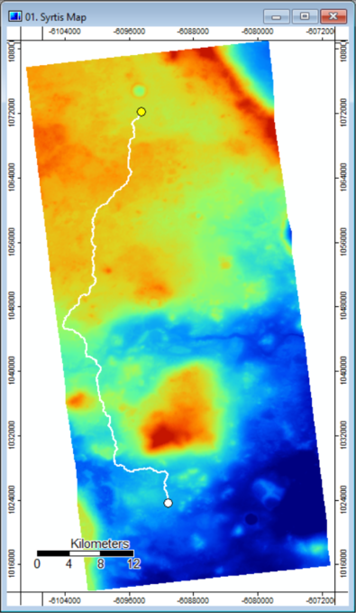
Under the “Data” tab, locate the “Profile Line [Accumulated Cost]” vector feature, and double click it to add it to the map. With the two points, the DTM and the profile line on the map, we now have the optimal path, based on the slope, that the rover could take between the start and end points. |
|||
[[File:Reclassify_window.png]] |
|||
Congratulations! You have now completed a basic least cost path analysis using DTM-derived terrain products. While this process was conducted using data from Mars, the procedure outlined above can be applied to any DTM or DEM. |
|||
==='''Accumulation Cost'''=== |
|||
[[Image:Final_map_with_least_cost_line.PNG|395px]] |
|||
An accumulation cost is necessary for Least Cost Path, here the values created above will be used for this step. By going into Geoprocessing>>Grid>>Cost Analysis>>Accumulated Cost(Isotropic) within this window: |
|||
The next section will elaborate on some tools and options for performing more complex cost-path analyses. |
|||
- Set the Grid system |
|||
=='''Advanced Cost Path Analysis Theory'''== |
|||
- The Cost Grid, in this case the reclassified slope layer |
|||
The process described above covers all of the basic steps required to perform a cost path analysis, but only begins to cover the details of complex cost path analyses as it only used on input for the cost surface. |
|||
- Set the destination points, the Kriging of the points |
|||
In the above rover example, the analysis assumes that slope is the single most important factor in determining the difficulty of the path chosen. However, just like Earth, there is more to the surface of Mars than simply the slope of the terrain. In order to get a more complete picture and more accurate assessment of the problem at hand, more data needs to be included. |
|||
In the rover example worked through above, additional data that would be relevant to the analysis could include surface material, surface roughness and aspect among others. |
|||
- The threshold for destination route, 0 was selected |
|||
When incorporating multiple datasets into the analysis, like the ones mentioned above, new factors need to be considered. The most notable factors are: |
|||
- How to assign costs/standardize all datasets |
|||
- Ensure that you create an accumulation cost and Closest point |
|||
- How to combine all datasets into one cost surface |
|||
[[File:Accumulation_Cost.png]] |
|||
These two factors are the most subjective and will vary the most between different applications and scenarios. In addition to being the most subjective elements, they are the most critical elements and can dramatically alter the outcomes of the analysis. As such, the methods used to represent data within the analysis are vital. |
|||
==='''Least Cost Path'''=== |
|||
One common method is to pick a common arbitrary scale along which to define the cost for each layer, such as a scale from 1 to 5, or 1 to 1000, depending on the granularity of cost is desired. Each layer can then be reclassified to match this cost scale and be compared to each other. |
|||
Alternatively, each layer can be reclassified such that they represent a measurable cost, such as dollars, fuel consumption or even time per unit area or length. |
|||
Either of these options make it such that layers can be directly compared to one another. |
|||
Once costs have been assigned to each data layer, the next challenge is figuring out which method to use to combine them into one cost surface. |
|||
The method used for combining data sets into a final cost surface is partially dependent on how costs were assigned to each data layer. Similarly to assigning costs, there are two main ways to combine data: |
|||
- Additive combination |
|||
Finally, finish the least cost path, by going into Geoprocessing>>Analysis>>Cost Analysis>> Least Cost Paths; |
|||
- Linear-weighted combination |
|||
- Select the grid system |
|||
Additive combination is simply adding all cost data layers into one, which is to be used as the base of the analysis. This method is the simplest and works well if all cost layers have similar influence or if the data are classed such that they represent measurable units rather than arbitrary ones. |
|||
- Within Accumulation Cost use the Accumulation Cost layer created above, |
|||
Linear-weighted combination involves assigning each layer a relative importance (generally expressed as a fraction of 1), such that the final cost layer is most influenced by the data with higher relative importance. This method is well suited to data that has a common scale and allows for easier fine-tuning of the cost model. |
|||
- Within Values select the nessecary values, in this case Slope was chosen. |
|||
The common theme with increasing the complexity of cost-path analyses is the high degree of subjectivity and application-specific methods required. This section is meant to be an introduction to these methods and is by no means an exhaustive list. |
|||
- The source points are the original point layer created at the begining of this tutorial |
|||
[[File:Least_Cost_Paths.png]] |
|||
'''More in depth research required''' |
|||
To fully understand what is happening and what selected process would work best for your DEM, readings should be done to see what each tool is and how to work on your selected file [http://www.saga-gis.org/saga_module_doc/2.1.3/a2z.html Full Module Index], as well as aids from other tutorials preforming a different method of cost path. |
|||
=Conclusion= |
=Conclusion= |
||
This tutorial showed the basic steps that are needed to perform a cost path analysis |
This tutorial showed the basic steps that are needed to perform a least cost path analysis using SAGA GIS. In addition, it introduced some theory behind performing more complex cost-path analyses. The world of distance analysis in GIS is complex and can be used in creative ways for a wide variety of applications. |
||
=References= |
=References= |
||
Dominoc925's Blog, How to digitise a new shape object in SAGA GIS, http://dominoc925.blogspot.com/2011/01/how-to-digitize-new-shape-object-in.html |
|||
Sohail Dham and Colin Doucette. Exploring Hydrological Analyses, http://gracilis.carleton.ca/CUOSGwiki/index.php/Exploring_Hydrological_Analyses_using_SAGA_GIS/ |
|||
Sohail Dham and Colin Doucette. Exploring Hydrological Analyses, http://gracilis.carleton.ca/CUOSGwiki/index.php/Exploring_Hydrological_Analyses_using_SAGA_GIS |
|||
Saga Library website, http://www.saga-gis.org/ |
Saga Tool Library website, http://www.saga-gis.org/saga_tool_doc/index.html |
||
Amanda Briney, Overview of Least Cost Path Analysis. https://www.gislounge.com/overview-least-cost-path-analysis/ |
|||
Saga Cost Path, http://sourceforge.net/projects/saga-gis/files/SAGA%20-%20Documentation/Tutorials/Least_Cost_Path_Analysis_Tutorial/ |
|||
SAGA GIS Tutorials, Reclassification. https://sagatutorials.wordpress.com/reclassification/ |
|||
Kim Cimmery(2013),Tutorial: Using SAGA for Least Cost Path Analysis,http://download2.polytechnic.edu.na/pub4/sourceforge/s/sa/saga-gis/SAGA%20-%20Documentation/Tutorials/Least_Cost_Path_Analysis_Tutorial/LCPAtutorial.pdf |
|||
Latest revision as of 18:12, 20 December 2018
Purpose
This tutorial aims to provide step-by-step instructions for completing cost-path analysis within SAGA. The basic analysis will use tools from the following built-in libraries: "Grid", "Shape" and "Terrain Analysis". A more advanced analysis will further explore tools within the Grid library. By the end, this tutorial will have shown you how to use SAGA’s built-in tools to perform a cost-path analysis using a Mars DTM and be exposed to more advanced techniques to enhance the basic cost-path analysis.
Introduction
SAGA
SAGA is an open source program for GIS that has a lot of capability in geoscientific analysis and has been designed for effective implementation of spatial algorithms. It features an extensive suite of tools covering raster data (called Grid data within SAGA) and operations, imagery processing, vector processing as well as some ecological and geomorphological simulations, to name a few. More information can be found at their homepage, and the latest version of the software can be downloaded from SourceForge. This tutorial uses SAGA v6.4.0.
To see more CUOSG tutorials that have used SAGA GIS, click here
Cost-Path Analysis
Cost-path Analysis is a GIS tool used for distance analysis and is primarily used for determining the most efficient route between two points. The strength of cost path analysis is its flexibility in modelling applications as it is only limited by what costs can be assigned to travel a distance. As a result, cost path analysis can be used in a variety of applications, and has been used to determine the best routes for power transmission lines, developing walking paths, determining ecological corridors for wildlife movement as well as modelling fire spread and flooding.
More details about cost path analysis can be found here.
Background and Data
This tutorial will explore the Northeast Syrtis region of Mars, which refers to the northeast area of Syrtis Planum Major quadrangle, which is a candidate landing spot for the Mars 2020 rover mission. As part of the preparation for the mission, stereo images of the potential landing site were taken by NASA’s Mars Reconnaissance Orbiter. The images were then used to create a digital terrain model (DTM), with the primary objective of being used in the rover mission’s Entry, Descent and Landing (EDL) simulations. The DTM of NE Syrtis (download here) is made available by the USGS Astrogeology Science Center.
For our analysis, we will be using the DTM as a base to determine a hypothetical path for the rover once it has landed.
A crucial element to note in this analysis is the type of coordinate system required. Any cost path analysis requires a projected coordinate system, which measures distance in units of distance (such as meters or feet), rather than a geographic coordinate system which uses angular units (degrees or radians). In this way, the analysis represents a cost associated with a consistent distance/area rather than angles, which vary in size as distance to the poles vary. Since we are using data from another planet, special attention must be given to the coordinate system. Fortunately, the DTM used in this example comes projected in an appropriate coordinate system and is ready for our analysis.
Methods
Basic Cost Path Analysis
Uploading Data into SAGA
The first step of the process is to download the DTM. The DTM of NE Syrtis comes in a TIFF (.tif) file format, which is a common file type for raster data in geospatial analysis. Once the file is downloaded, open the SAGA software. Start with an empty startup project.
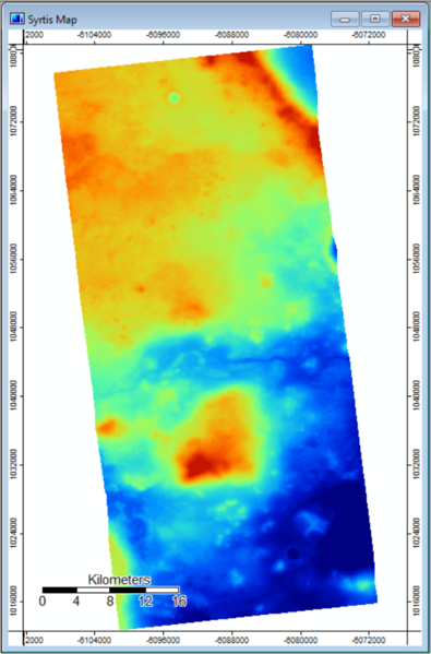
To import the DTM, go to “File >> Grid >> Load” and navigate to where you stored the DTM. Click Open. The file might take a little while to load. Next, double click the file you just imported. A map should appear, and look like the image below.
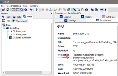
The presence of the scale bar with units in Kilometers indicates that we have a projection suitable projection. To check the details, navigate to the “Description” tab in the properties window, and check the Projection. It should say “EquirectangularMars”, with its parameters below.
Now we’ll rename a few things to make the analysis process smoother.
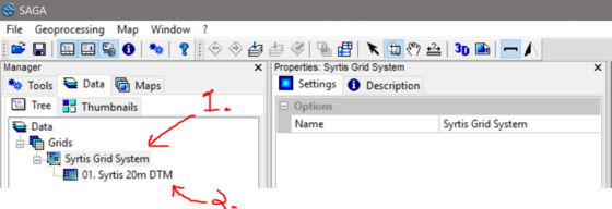
First we’ll rename the Grid System, the first entry under “Grids” in the data tab (1. in photo below). Under the “Settings” tab in the Properties window, click to the right of the “Name” field. I chose to rename it “Syrtis Grid System”.
Next we’ll do the same for the DTM itself. Click on the DTM layer (2. in photo below), then repeat the above process. I named the DTM “Syrtis 20m DTM”.
Now we’re ready to continue with the analysis.
Creating Points
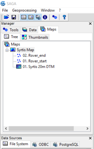
To perform our cost-path analysis, we need to create a starting point and ending point for our path. To do so we will need to create two new vector layers.
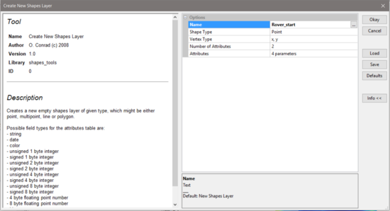
To create a vector layer, we’ll use the geoprocessing tools. Navigate to “Geoprocessing >> Shapes >> Construction >> Create new “Shapes layer”. Check that the Shape Type is Points, then change the name to “Rover_start”. Click Okay.
Repeat the process to create the “Rover_end” layer.
Under the Data Tab in the Manager on the left, you should see the three elements we have so far. Double click each point shape to add it to the map. The map panel should look like the following.
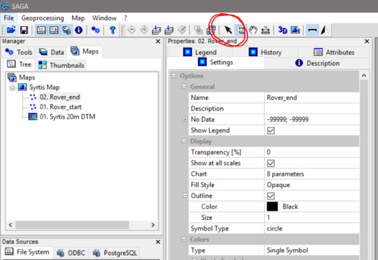
Next we need to create the points on our map. To do so, click on the layer you want to edit in the Maps tab. Right click, go to “Edit >> Add Shape”. From the top menu bar, click on the arrow pointer, called the “Action Tool”.
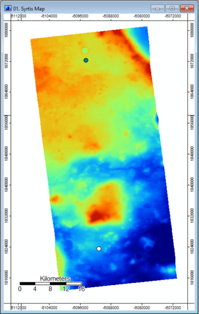
Next, left-click somewhere in the top half of the map; this will be our starting point. When you’re happy with the location, right-click and select “Edit Selection” and click “Yes” on the window that pops up.
Repeat for the end point, this time placing the point near the bottom of the map. You should now have two points on your map.
We are now ready to move on to the Terrain Analysis portion of the analysis.
Terrain Analysis
This portion of the analysis turns our DTM into a set of derivative terrain products from which we will base our cost path analysis from. SAGA has a convenient tool that can calculate slope, aspect and curvature within a single window.
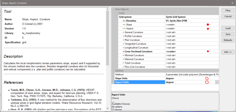
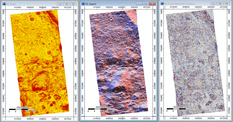
To create the terrain products, go to “Geoprocessing >> Terrain Analysis >> Morphometry >> Slope, Aspect, Curvature”. The inputs are “Syrtis Grid System” for the grid system and “Syrtis 20m DTM” for the elevation. To get our outputs, we need to select “<create>” on the following elements: “Slope”, “Aspect” and “Cross-Sectional Curvature”. We will also change the units for both Slope and Aspect to degrees.
When all the options have been correctly set, click Okay. The outputs can now be found in the Data tab of the Manager. Below is an image of the three outputs.
Reclassify
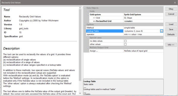
We have created some terrain products, but they aren’t particularly meaningful for use in cost path analysis right away. We will be using the Slope layer as the basis of our analysis and we will reclassify some of the values to better represent the difficulty of crossing varied terrain. To start reclassifying, navigate to “Geoprocessing >> Grid >> Values >> Reclassify Grid Values”. In the tool menu, select the following inputs: “Syrtis Grid System” for the grid system, “Slope” for the grid. Next, we need to define the method for reclassifying the raster. Under Method, select “simple table”.
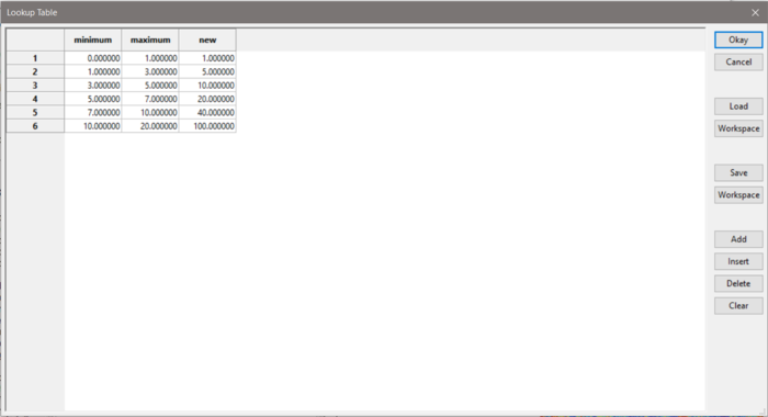
On the next line below, click the three dots on the right-hand line of “Lookup Table”. This should open a new window. Add some lines and enter the values to look like the following photo.
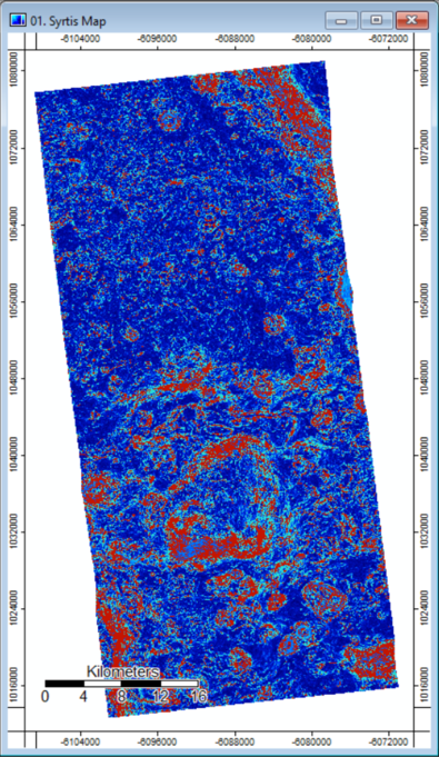
When happy with the values, click Okay on the Lookup Table window, then Okay on the tool. Below is a photo of the reclassified slope layer.
The values selected for reclassification were arbitrarily determined and will be sufficient for this process. However, determining appropriate cost values, as will be discussed later, is one of the most difficult elements of cost path analysis.
Accumulation Cost
Now that we have created our terrain products and reclassified our slope data into something meaningful, we are ready to begin the cost-path analysis. The first step is to create an accumulation cost surface. Given a vector point (our destination point), this tool returns a surface that represents how “expensive” it is to travel away from the given input point. This will be the input for the final step of our least cost path analysis.
To create the accumulation cost surface, navigate to “Geoprocessing >> Grid >> Analysis >> Cost Analysis >> Accumulation Cost”. The inputs should be "Syrtis Grid System" for the grid system, "Slope_reclassified" for the local cost, and "Rover_end" as the destination point. Once this is done, click Okay. The output will show up on the “Data” tab labeled “Accumulated Cost”. Double click it to add it to the map.
Below is an image of the accumulation cost raster. It shows areas of low cost in blue (near the end point) and areas with increasing cost in red.
Now we move on to complete the last step in our analysis.
Least Cost Path
To complete our analysis and see the final product, we will finally run the Least Cost Path analysis tool. It can be found under “Geoprocessing >> Grid >> Analysis >> Cost Analysis >> Least Cost Path”
The inputs are “Syrtis Grid System” for the grid system and “Accumulated Cost” for the accumulated cost surface. The Source Points is our “Rover_start” point file. Click Okay when ready.
Under the “Data” tab, locate the “Profile Line [Accumulated Cost]” vector feature, and double click it to add it to the map. With the two points, the DTM and the profile line on the map, we now have the optimal path, based on the slope, that the rover could take between the start and end points.
Congratulations! You have now completed a basic least cost path analysis using DTM-derived terrain products. While this process was conducted using data from Mars, the procedure outlined above can be applied to any DTM or DEM.
The next section will elaborate on some tools and options for performing more complex cost-path analyses.
Advanced Cost Path Analysis Theory
The process described above covers all of the basic steps required to perform a cost path analysis, but only begins to cover the details of complex cost path analyses as it only used on input for the cost surface. In the above rover example, the analysis assumes that slope is the single most important factor in determining the difficulty of the path chosen. However, just like Earth, there is more to the surface of Mars than simply the slope of the terrain. In order to get a more complete picture and more accurate assessment of the problem at hand, more data needs to be included.
In the rover example worked through above, additional data that would be relevant to the analysis could include surface material, surface roughness and aspect among others. When incorporating multiple datasets into the analysis, like the ones mentioned above, new factors need to be considered. The most notable factors are:
- How to assign costs/standardize all datasets
- How to combine all datasets into one cost surface
These two factors are the most subjective and will vary the most between different applications and scenarios. In addition to being the most subjective elements, they are the most critical elements and can dramatically alter the outcomes of the analysis. As such, the methods used to represent data within the analysis are vital. One common method is to pick a common arbitrary scale along which to define the cost for each layer, such as a scale from 1 to 5, or 1 to 1000, depending on the granularity of cost is desired. Each layer can then be reclassified to match this cost scale and be compared to each other. Alternatively, each layer can be reclassified such that they represent a measurable cost, such as dollars, fuel consumption or even time per unit area or length. Either of these options make it such that layers can be directly compared to one another.
Once costs have been assigned to each data layer, the next challenge is figuring out which method to use to combine them into one cost surface. The method used for combining data sets into a final cost surface is partially dependent on how costs were assigned to each data layer. Similarly to assigning costs, there are two main ways to combine data:
- Additive combination
- Linear-weighted combination
Additive combination is simply adding all cost data layers into one, which is to be used as the base of the analysis. This method is the simplest and works well if all cost layers have similar influence or if the data are classed such that they represent measurable units rather than arbitrary ones.
Linear-weighted combination involves assigning each layer a relative importance (generally expressed as a fraction of 1), such that the final cost layer is most influenced by the data with higher relative importance. This method is well suited to data that has a common scale and allows for easier fine-tuning of the cost model.
The common theme with increasing the complexity of cost-path analyses is the high degree of subjectivity and application-specific methods required. This section is meant to be an introduction to these methods and is by no means an exhaustive list.
Conclusion
This tutorial showed the basic steps that are needed to perform a least cost path analysis using SAGA GIS. In addition, it introduced some theory behind performing more complex cost-path analyses. The world of distance analysis in GIS is complex and can be used in creative ways for a wide variety of applications.
References
Dominoc925's Blog, How to digitise a new shape object in SAGA GIS, http://dominoc925.blogspot.com/2011/01/how-to-digitize-new-shape-object-in.html
Sohail Dham and Colin Doucette. Exploring Hydrological Analyses, http://gracilis.carleton.ca/CUOSGwiki/index.php/Exploring_Hydrological_Analyses_using_SAGA_GIS
Saga Tool Library website, http://www.saga-gis.org/saga_tool_doc/index.html
Amanda Briney, Overview of Least Cost Path Analysis. https://www.gislounge.com/overview-least-cost-path-analysis/
SAGA GIS Tutorials, Reclassification. https://sagatutorials.wordpress.com/reclassification/
