Difference between revisions of "Remote Sensing Analysis in QGIS"
m (→Conclusions) |
|||
| (38 intermediate revisions by 3 users not shown) | |||
| Line 5: | Line 5: | ||
==Obtaining Data and Software== |
==Obtaining Data and Software== |
||
To begin, the user must download the most recent version of QGIS. The current version is QGIS 3. |
To begin, the user must download the most recent version of QGIS. The current version is QGIS 3.8.3. 'Zanzibar', originally released on September 13th 2019. The most up to date version can be downloaded using the following [https://www.qgis.org/en/site/forusers/download.html]. Select your operating system and ensure that you download the proper version (32-Bit or 64-Bit for windows machines). |
||
Landsat imagery is preprocessed and made publically available by the United States Geological Survey (USGS). Images can be browsed and downloaded through the [https://earthexplorer.usgs.gov/ EarthExplorer] application. To get access to the imagery you need to create an account. |
Landsat imagery is preprocessed and made publically available by the United States Geological Survey (USGS). Images can be browsed and downloaded through the [https://earthexplorer.usgs.gov/ EarthExplorer] application. To get access to the imagery you need to create an account. |
||
| Line 32: | Line 32: | ||
'''Step 4:''' Finally, the results of our search can be seen under the '''Results''' tab. We can select to show the footprint of this image, view a preview and download any of the resulting images. For this tutorial, download the scene from May 15th 2013. Snow in the valley has mostly melted but large icings are still present, making it ideal for our purposes. |
'''Step 4:''' Finally, the results of our search can be seen under the '''Results''' tab. We can select to show the footprint of this image, view a preview and download any of the resulting images. For this tutorial, download the scene from May 15th 2013. Snow in the valley has mostly melted but large icings are still present, making it ideal for our purposes. After downloading the pictures make sure that you unzip the images twice in your Explorer. |
||
[[File:SearchResults.jpg|800px]] |
[[File:SearchResults.jpg|800px]] |
||
==Landsat 8 Bands== |
|||
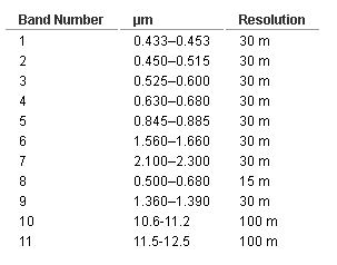
Landsat 8 image has 11 bands, but only bands 1 - 4 and 8 are visible light. The following picture is all Landsat 8 bands and relevant wavelengths. |
|||
[[File:Band wavelength.JPG|400px]] |
|||
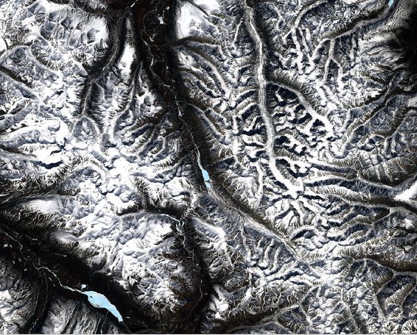
To create a true colour image, set Band 4-3-2 as RGB band respectively. |
|||
To create a false colour composite for the study area (mostly Land and water), set band 5-6-4 as RGB band respectively. Similarly, if you are going to produce a false colour composite image for urban area, set band 7-6-4 as RGB band respectively. |
|||
For this tutorial, we are only going to create true colour image. |
|||
[[File:True colour image.JPG|600px]] |
|||
==Loading Imagery and Atmospheric Correction== |
==Loading Imagery and Atmospheric Correction== |
||
| Line 41: | Line 52: | ||
We can now begin working with the data in QGIS. Begin by loading the different landsat bands into QGIS. At the top of the user surface press '''Layer''' then '''Add Layer''' and choose '''Add Raster Layer'''. |
|||
[[File:RasterSymbol.jpg]] |
[[File:RasterSymbol.jpg]] |
||
| Line 49: | Line 60: | ||
While the data obtained from EarthExplorer is very good, it still needs some correction applied in order to remove the haze and scattering that occurs when images are taken through |
While the data obtained from EarthExplorer is very good, it still needs some correction applied in order to remove the haze and scattering that occurs when images are taken through Earth's atmosphere. To do this, we will utilize the '''Semi-automatic Classification Plugin''', or '''SCP''' within QGIS. Semi-automatic Classification Plugin is a free open source add-on for QGIS, and we can use it to do remote sensing analysis, and classification (either unsupervised or supervised). You can also use it to do land cover change analysis, and image classification accuracy reporting. The Semi-Automatic Classification Plugin can also do remote sensing analysis for other types of satellite imagery, and you can also directly download satellite image from this plugin. Semi-Automatic Classification Plugin supports all versions of Landsat satellite image, Sentinel-2, Sentinel-3, ASTER, and MODIS. |
||
| Line 69: | Line 80: | ||
Our imagery is now ready to work with! |
Our imagery is now ready to work with! |
||
==Calculating Indices in Raster Calculator== |
==Calculating Indices in Raster Calculator== |
||
| Line 83: | Line 92: | ||
To begin, open the '''Raster Calculator''' by navigating to the '''Raster''' menu at the top of the page. |
To begin, open the '''Raster Calculator''' by navigating to the '''Raster''' menu at the top of the page. |
||
The first index we will calculate is the '''NDSI''', or the Normalized Difference Snow Index. This is an index designed to tease out snow from the landscape. Our scene still has a lot of snow present on mountain peaks, so there should be a lot of snow present in the scene. |
The first index we will calculate is the '''NDSI''', or the Normalized Difference Snow Index. This is an index designed to tease out snow from the landscape. Our scene still has a lot of snow present on mountain peaks, so there should be a lot of snow present in the scene. Snow and cloud have similar reflectance before SWIR band, however, snow reflectance drops to 5% in SWIR but cloud reflectance increases to 60%. Therefore band 6 is required to calculate NDSI to distinguish snow from clouds. |
||
The formula for NDSI is ((Band 3 - Band 6) / (Band 3 + Band 6)), and can be entered into the raster calculator as seen below. Ensure that the expression is valid and that you have set the appropriate path for the output file. To identify your file later easily, I suggest naming it NDSI.tif. |
The formula for NDSI is ((Band 3 - Band 6) / (Band 3 + Band 6)), and can be entered into the raster calculator as seen below. Ensure that the expression is valid and that you have set the appropriate path for the output file. To identify your file later easily, I suggest naming it NDSI.tif. |
||
[[File:Calculate_NDSI.JPG|800px]] |
[[File:Calculate_NDSI.JPG|800px]] |
||
| Line 107: | Line 116: | ||
The output should give two classes of values ; a value of '''1''' where the conditions were met (aka snow is present) and '''0''' where there is no snow. We can now reclassify this output to isolate the class containing snow using the '''Translate (Convert Format)''' tool, found under '''Raster, Conversion, Translate'''. Be sure to select the correct Input Layer. Enter '''0''' in the field under ''Assign a |
The output should give two classes of values ; a value of '''1''' where the conditions were met (aka snow is present) and '''0''' where there is no snow. We can now reclassify this output to isolate the class containing snow using the '''Translate (Convert Format)''' tool, found under '''Raster, Conversion, Translate'''. Be sure to select the correct Input Layer. Enter '''0''' in the field under ''Assign a specified nodata value to output bands''. Define the Output data type as '''Byte'''. This will classify everything that did not meet the conditions of the raster calculator to NoData, or blank. Also be sure to specify an appropriate output folder. The easiest way is to '''save it as a file''' and not as a temporary file. Unfortunately, in the user surface the layer will be called ''Converted'' instead of the name you choose. But when you navigate with your mouse to the layer you will see the name you have chosen. |
||
| Line 130: | Line 139: | ||
[[File: |
[[File:Calc_MDII.JPG|800px]] |
||
| Line 140: | Line 149: | ||
We can reclassify this output using the '''Translate''' tool again, except 1 equates to areas of ice and 0 has no ice instead of snow. click the '''No Data''' button and set the value to 0. This will classify everything that did not meet the conditions of the raster calculator to NoData, or blank. Also be sure to specify an appropriate output folder, possibly in an '''Indices''' folder alongside the NDSI output for organizational purposes. |
We can reclassify this output using the '''Translate''' tool again, except 1 equates to areas of ice and 0 has no ice instead of snow. click the '''No Data''' button and set the value to 0. This will classify everything that did not meet the conditions of the raster calculator to NoData, or blank. Also be sure to specify an appropriate output folder, possibly in an '''Indices''' folder alongside the NDSI output for organizational purposes. |
||
The output file should look like this: |
|||
[[File:Only ice.JPG|600px]] |
|||
===NDWI=== |
===NDWI=== |
||
| Line 151: | Line 163: | ||
Again, we can select a range of values from this index that best represent water. In this case, the values corresponding to water are greater than -0.3 but less than 0. Then we can reclassify this output using the same steps as before to create a raster file containing areas of water. Some error stems from the abundant mountain snow in our scene, which is unavoidable due to the spectral properties of melting snow. |
Again, we can select a range of values from this index that best represent water. In this case, the values corresponding to water are greater than -0.3 but less than 0. Then we can reclassify this output using the same steps as before to create a raster file containing areas of water. Some error stems from the abundant mountain snow in our scene, which is unavoidable due to the spectral properties of melting snow. |
||
[[File:Extract_water.JPG|400px]] |
|||
The output file should look like this: |
|||
[[File:Justwater.JPG|600px]] |
|||
To fix the error above, we are going to use NDWI value '''greater than 0.5''' instead of greater than -0.3 but less than 0. |
|||
The output file should look like this: |
|||
[[File:Water final.JPG|600px]] |
|||
==Final Products== |
==Final Products== |
||
For display and reference purposes, we can render our Landsat scene to show standard RGB colours. This can be done using the '''Band Stack''' function within the semi-automatic classification plugin. You can find the tool at the top of the user surface. The band designations for '''RGB''' in Landsat 8 are '''4,3,2''' respectively. |
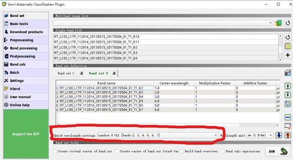
For display and reference purposes, we can render our Landsat scene to show standard RGB colours. This can be done using the '''Band Stack''' function within the semi-automatic classification plugin. For Landsat - 8 image, choose band 2 - 7 for the Band Stack image and select Landsat 8 OLI in the Quick wavelength settings. You can find the tool at the top of the user surface. The band designations for '''RGB''' in Landsat 8 are '''4,3,2''' respectively. |
||
[[File:Inkedsetting LI.jpg|600px]] |
|||
The band designations for '''RGB''' in Landsat 8 are '''4,3,2''' respectively. |
|||
| Line 166: | Line 194: | ||
After clicking the symbol, at the right side of your screen appears the '''Layer Styling''' window as you see in the following image. There you can select the layers and allocate them colours. Because you may have three layers called ''Converted'' be aware |
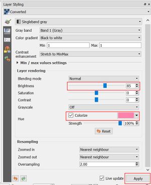
After clicking the symbol, at the right side of your screen appears the '''Layer Styling''' window as you see in the following image. There you can select the layers and allocate them colours. Because you may have three layers called ''Converted'' be aware which ones you choose. Make sure you raise the brightness, otherwise you won't see the colours. |
||
[[File:Layer_Styling.JPG|300px]] |
[[File:Layer_Styling.JPG|300px]] |
||
| Line 174: | Line 202: | ||
[[File: |
[[File:Final product2.JPG|400px]] |
||
[[File:Final product.JPG|600px]] |
|||
==Other Indices: Operational Formulae== |
|||
The above tutorial introduced how to calculate water, snow, and ice indices. Other applications can use similar indices for other purposes. |
|||
If you have a study area that contains urban area or vegetation, you could use QGIS raster calculator to calculate NDVI, NDBI, and NDWI. |
|||
NDVI is the Normalized Difference Vegetation Index. If you are using Landsat 8 data, NDVI = (Band 5 - Band 4)/(Band 5 + Band 4). NDVI = 0.2 to 0.5 represent Shrubs and grasslands, and NDVI = 0.6 to 0.9 areas are dense vegetation. |
|||
NDBI is the Normalized Difference Built-up Index. NDBI = (Band 6 - Band 5)/(Band 6 + Band 5). Positive NDBI value correspond to build-up areas. |
|||
Unlike the NDWI above, NDWI can also calculate by (Band 5 - Band 6)/(Band 5 + Band 6). However, "Pure water neither reflects NIR nor SWIR - TEK, 2018", and NDWI are commonly used in moisture content in vegetation and soils. Therefore NDWI = (Band 5 - Band 6)/(Band 5 + Band 6) is rarely used. |
|||
==Conclusions== |
==Conclusions== |
||
This tutorial has showcased some of the remote sensing capabilities of QGIS in the context of scientific analysis. The products generated could be used to asses how icing distribution changes over time, calculations of water stored in icings or threat posed to local infrastructure. I hope this guide may empower those without the means to purchase expensive software to pursue scientific endeavors in the future. |
This tutorial has showcased some of the remote sensing capabilities of QGIS in the context of scientific analysis. The products generated could be used to asses how icing distribution changes over time, calculations of water stored in icings or threat posed to local infrastructure. I hope this guide may empower those without the means to purchase expensive software to pursue scientific endeavors in the future. |
||
If you are interested to get more knowledge about Remote Sensing I recommend the following books: |
|||
Lillesand, T., Kiefer, R., Chipman, J. (2015): Remote Sensing and image interpretation. Wiley, Hokboken. |
|||
Mårtensson, U., (2016): Remote Sensing and image interpretation. |
|||
Solimni, D. (2016): Understadning Earth Observation. Springer, Cham. |
|||
Latest revision as of 23:34, 28 October 2019
Contents
Introduction
Remote sensing is a broad discipline involving the observation of an object or phenomenon without physically interacting with it. In a remote sensing context, this generally involves the analysis of remotely sensed images from a variety of sources such as RADAR or multispectral satellite imagery. However, many commercially available remote sensing softwares can be very expensive and not accessible to the average user outside of major private or public institutions.
The purpose of this tutorial is to showcase the remote sensing capabilities of the free GIS software QGIS. To do this, we will be going through a workflow to delineate icings from Landsat imagery. Icings, thick masses of ice that build up through successive overflows, can endanger remote communities or vital infrastructure. The workflow was originally designed using expensive proprietary software such as ENVI and ArcGIS. By reproducing the finished products using free software, this tutorial hopes to demonstrate the capabilities of QGIS in a real scientific application.
Obtaining Data and Software
To begin, the user must download the most recent version of QGIS. The current version is QGIS 3.8.3. 'Zanzibar', originally released on September 13th 2019. The most up to date version can be downloaded using the following [1]. Select your operating system and ensure that you download the proper version (32-Bit or 64-Bit for windows machines).
Landsat imagery is preprocessed and made publically available by the United States Geological Survey (USGS). Images can be browsed and downloaded through the EarthExplorer application. To get access to the imagery you need to create an account.
In EarthExplorer, we need to narrow down the vast repository of data that is available. Firstly, we must filter the data to only include summer images. This increases our ability to extract icings from the landscape, as there is little to no snow left on the ground.
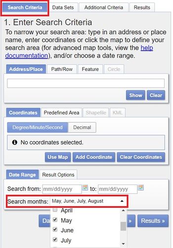
Step 1: Navigate to the Search Months dropdown menu at the bottom of the Search Criteria tab and unselect all months except May, June, July and August as seen in the screenshot below.
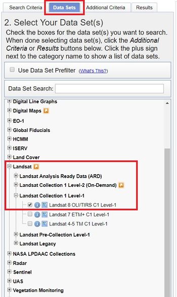
Step 2: For our purposes, we should use the imagery with the broadest spectral range. Launched in 2013, data from the Landsat 8 platform should be suitable. Select the Datasets tab at the top of the page and navigate to Landsat, Landsat Collection 1 Level-1 and select Landsat 8 OLI/TIRS C1 Level 1.
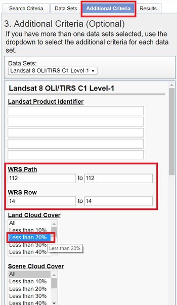
Step 3: We can now narrow down the search in even greater detail using the Additional Criteria tab. We need to find an area with visible icings, commonly near the bottom of mountain slopes at high latitudes, where the hydrological and climate conditions favor icing formation. Landsat missions split the earth up into a grid of paths and rows for easy image identification. After some searching, a scene with good icing potential can be found at path 112 row 14, corresponding to an area in Siberia. We can also choose to limit cloud cover to 20% in order to minimize noise in the imagery. Enter these criteria as shown below.
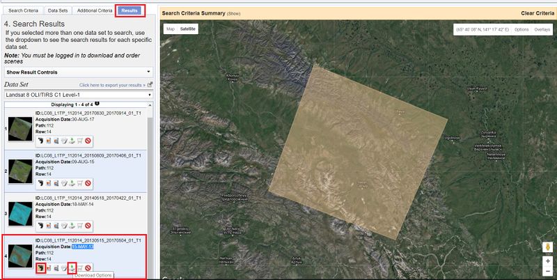
Step 4: Finally, the results of our search can be seen under the Results tab. We can select to show the footprint of this image, view a preview and download any of the resulting images. For this tutorial, download the scene from May 15th 2013. Snow in the valley has mostly melted but large icings are still present, making it ideal for our purposes. After downloading the pictures make sure that you unzip the images twice in your Explorer.
Landsat 8 Bands
Landsat 8 image has 11 bands, but only bands 1 - 4 and 8 are visible light. The following picture is all Landsat 8 bands and relevant wavelengths.
To create a true colour image, set Band 4-3-2 as RGB band respectively. To create a false colour composite for the study area (mostly Land and water), set band 5-6-4 as RGB band respectively. Similarly, if you are going to produce a false colour composite image for urban area, set band 7-6-4 as RGB band respectively. For this tutorial, we are only going to create true colour image.
Loading Imagery and Atmospheric Correction
We can now begin working with the data in QGIS. Begin by loading the different landsat bands into QGIS. At the top of the user surface press Layer then Add Layer and choose Add Raster Layer.
Semi-automatic Classification Plugin
While the data obtained from EarthExplorer is very good, it still needs some correction applied in order to remove the haze and scattering that occurs when images are taken through Earth's atmosphere. To do this, we will utilize the Semi-automatic Classification Plugin, or SCP within QGIS. Semi-automatic Classification Plugin is a free open source add-on for QGIS, and we can use it to do remote sensing analysis, and classification (either unsupervised or supervised). You can also use it to do land cover change analysis, and image classification accuracy reporting. The Semi-Automatic Classification Plugin can also do remote sensing analysis for other types of satellite imagery, and you can also directly download satellite image from this plugin. Semi-Automatic Classification Plugin supports all versions of Landsat satellite image, Sentinel-2, Sentinel-3, ASTER, and MODIS.
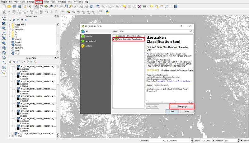
Navigate to the Plugins' menu at the top of the user and click Manage and Install Plugins. In the search bar, begin typing SEMI and the semi-automatic classification plugin will appear. Click the Install Plugin button on the bottom right begin using the plugin, as seen below.
Once the SCP is installed, activate it from the Manage and Install Plugins window. There should now be an SCP drop-down menu along the top of the user interface. This plugin contains a variety of different remote sensing tools beyond its classification abilities. Select SCP, Preprocessing, Landsat to open up the atmospheric correction window.
Once the window is open, enter the directory in which you've unzipped the Landsat files obtained from EarthExplorer into the Directory containing Landsat bands option. As this file should already contain the metadata file (.MTL) for the imagery, there is no need to specify its location. The metadata including date, elevation and the Earth to Sun distance should be automatically filled in.
After ensuring that all of the bands and metadata have been recognized by the plugin, check the Apply DOS1 atmospheric correction and click the Run button in the bottom right. You will be prompted to choose a directory for the output files, which should be named appropriately (eg. ATCOR).
Our imagery is now ready to work with!
Calculating Indices in Raster Calculator
The different bands of Landsat 8 correspond to different spectral wavelengths. By performing calculations on different combinations of bands, we can highlight specific features within a scene through the use of an index. The most commonly used index is most likely NDVI, or the Normalized Difference Vegetation Index, which is used to highlight areas of healthy vegetation. Using a similar concept, we will calculate various indices that highlight ice, snow and water in order to effectively extract icings from our scene.
NDSI
To begin, open the Raster Calculator by navigating to the Raster menu at the top of the page.
The first index we will calculate is the NDSI, or the Normalized Difference Snow Index. This is an index designed to tease out snow from the landscape. Our scene still has a lot of snow present on mountain peaks, so there should be a lot of snow present in the scene. Snow and cloud have similar reflectance before SWIR band, however, snow reflectance drops to 5% in SWIR but cloud reflectance increases to 60%. Therefore band 6 is required to calculate NDSI to distinguish snow from clouds.
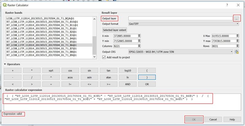
The formula for NDSI is ((Band 3 - Band 6) / (Band 3 + Band 6)), and can be entered into the raster calculator as seen below. Ensure that the expression is valid and that you have set the appropriate path for the output file. To identify your file later easily, I suggest naming it NDSI.tif.
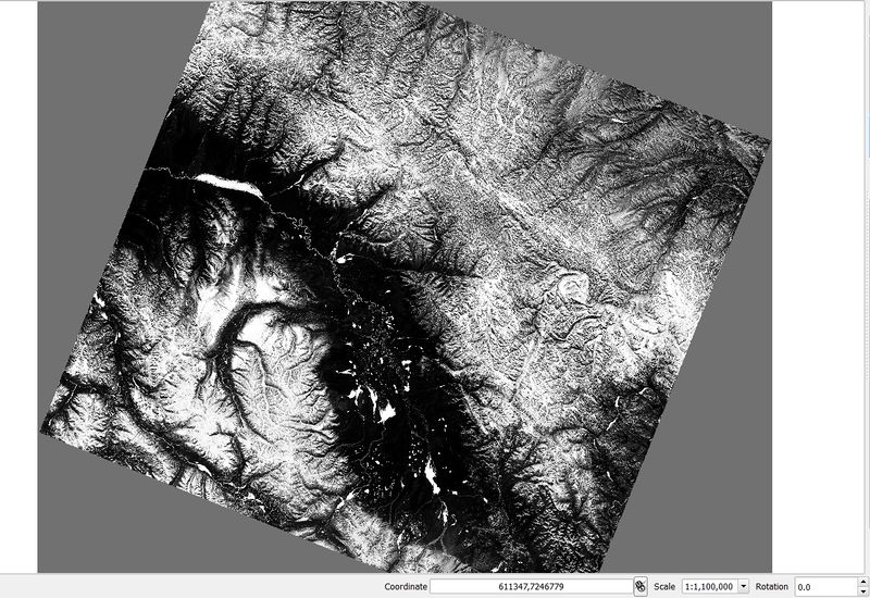
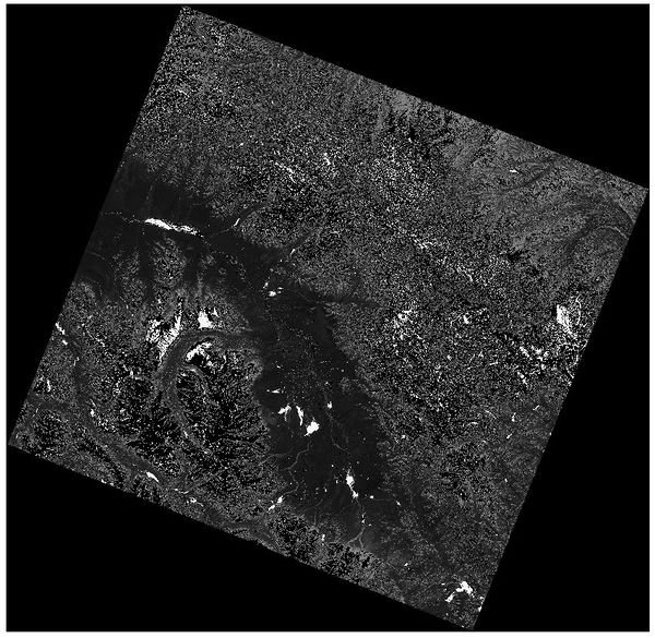
The output of this calculation should look like the image below.
From this output, we must now extract the range of values that correspond to snow. Using the Identify button along the top of the user interface.
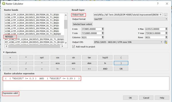
We can assess the values of the index and come up with an appropriate range of values that can be considered snow. In this case, values over 0.3 and less than 0.89 can be considered snow.
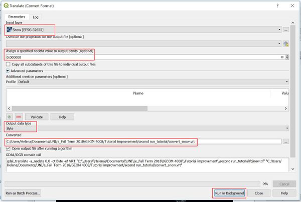
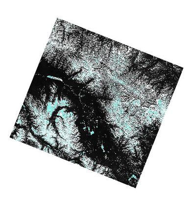
The output should give two classes of values ; a value of 1 where the conditions were met (aka snow is present) and 0 where there is no snow. We can now reclassify this output to isolate the class containing snow using the Translate (Convert Format) tool, found under Raster, Conversion, Translate. Be sure to select the correct Input Layer. Enter 0 in the field under Assign a specified nodata value to output bands. Define the Output data type as Byte. This will classify everything that did not meet the conditions of the raster calculator to NoData, or blank. Also be sure to specify an appropriate output folder. The easiest way is to save it as a file and not as a temporary file. Unfortunately, in the user surface the layer will be called Converted instead of the name you choose. But when you navigate with your mouse to the layer you will see the name you have chosen.
The output file should look like this:
MDII
The second index we will calculate is the MDII, or the Maximized Difference ICE Index. This is an index designed to tease out pure ice from the landscape. The scene we chose is in early summer, where ice is still at its maximum extent but most surface snow in the valleys has melted. This should help to reduce noise in the final image.
Reopen the Raster Calculator from the top menu
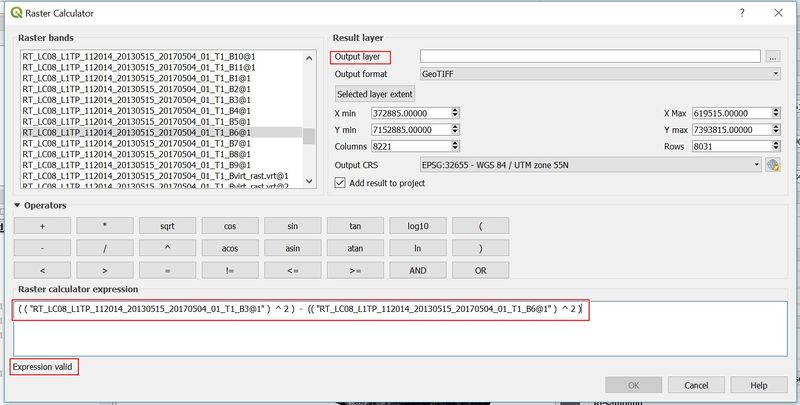
The formula for MDII is ((Band 3)^2) - (Band 6)^2)), and can be entered into the raster calculator as seen below. Ensure that the expression is valid and that you have set the appropriate path for the output file.
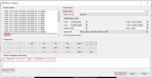
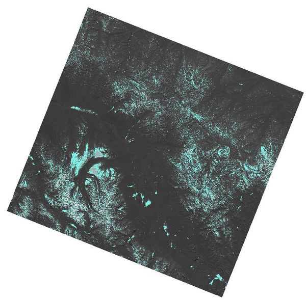
The output of this file is in the same structure as the NDSI index in the previous section. From this output, we must now extract the range of values that correspond to pure ice. Using the Identify button along the top of the user interface, we can assess the values of the index and come up with an appropriate range of values that can be considered ice. In this case, values over 0.25 and less than 0.5 can be considered ice.
We can reclassify this output using the Translate tool again, except 1 equates to areas of ice and 0 has no ice instead of snow. click the No Data button and set the value to 0. This will classify everything that did not meet the conditions of the raster calculator to NoData, or blank. Also be sure to specify an appropriate output folder, possibly in an Indices folder alongside the NDSI output for organizational purposes.
The output file should look like this:
NDWI
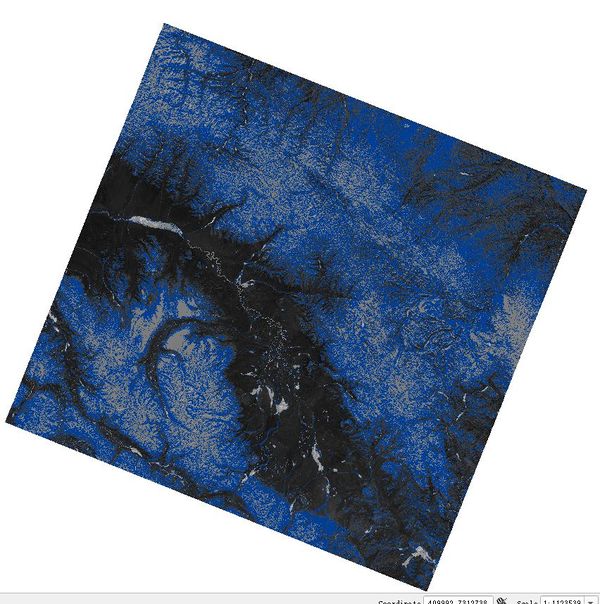
The final index that will be calculated is the NDWI, or the Normalized Difference Water Index. By extracting water from the image we can mask out bodies of ice that occur over water, thereby ensuring that all ice mapped occurs over land. This type of ice is of the most concern to this area of study, as ice spilling out over the land poses the largest potential threat to infrastructure in vulnerable areas. NDWI can be calculated using the expression ((Band 3 - Band 5) / (Band 3 + Band 5)).
Again, we can select a range of values from this index that best represent water. In this case, the values corresponding to water are greater than -0.3 but less than 0. Then we can reclassify this output using the same steps as before to create a raster file containing areas of water. Some error stems from the abundant mountain snow in our scene, which is unavoidable due to the spectral properties of melting snow.
The output file should look like this:
To fix the error above, we are going to use NDWI value greater than 0.5 instead of greater than -0.3 but less than 0.
The output file should look like this:
Final Products
For display and reference purposes, we can render our Landsat scene to show standard RGB colours. This can be done using the Band Stack function within the semi-automatic classification plugin. For Landsat - 8 image, choose band 2 - 7 for the Band Stack image and select Landsat 8 OLI in the Quick wavelength settings. You can find the tool at the top of the user surface. The band designations for RGB in Landsat 8 are 4,3,2 respectively.
The band designations for RGB in Landsat 8 are 4,3,2 respectively.
Once rendered, we can turn on the three extracted layers in order to see the icings clearly. To edit the colors, you can find the layers panel at the top of your layers window.
After clicking the symbol, at the right side of your screen appears the Layer Styling window as you see in the following image. There you can select the layers and allocate them colours. Because you may have three layers called Converted be aware which ones you choose. Make sure you raise the brightness, otherwise you won't see the colours.
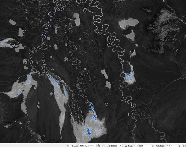
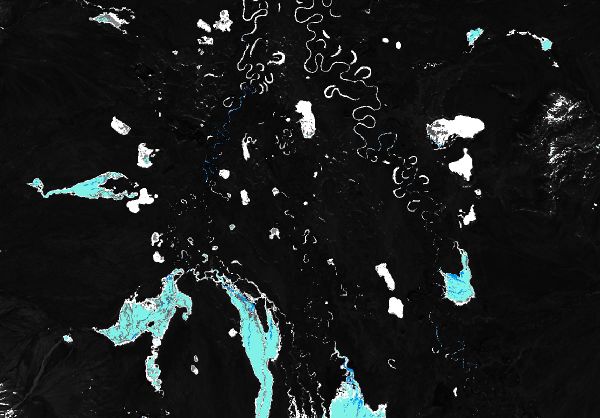
Your final picture could look like this (depends on the colours yo have seleceted).
Other Indices: Operational Formulae
The above tutorial introduced how to calculate water, snow, and ice indices. Other applications can use similar indices for other purposes. If you have a study area that contains urban area or vegetation, you could use QGIS raster calculator to calculate NDVI, NDBI, and NDWI.
NDVI is the Normalized Difference Vegetation Index. If you are using Landsat 8 data, NDVI = (Band 5 - Band 4)/(Band 5 + Band 4). NDVI = 0.2 to 0.5 represent Shrubs and grasslands, and NDVI = 0.6 to 0.9 areas are dense vegetation.
NDBI is the Normalized Difference Built-up Index. NDBI = (Band 6 - Band 5)/(Band 6 + Band 5). Positive NDBI value correspond to build-up areas.
Unlike the NDWI above, NDWI can also calculate by (Band 5 - Band 6)/(Band 5 + Band 6). However, "Pure water neither reflects NIR nor SWIR - TEK, 2018", and NDWI are commonly used in moisture content in vegetation and soils. Therefore NDWI = (Band 5 - Band 6)/(Band 5 + Band 6) is rarely used.
Conclusions
This tutorial has showcased some of the remote sensing capabilities of QGIS in the context of scientific analysis. The products generated could be used to asses how icing distribution changes over time, calculations of water stored in icings or threat posed to local infrastructure. I hope this guide may empower those without the means to purchase expensive software to pursue scientific endeavors in the future.
If you are interested to get more knowledge about Remote Sensing I recommend the following books:
Lillesand, T., Kiefer, R., Chipman, J. (2015): Remote Sensing and image interpretation. Wiley, Hokboken.
Mårtensson, U., (2016): Remote Sensing and image interpretation.
Solimni, D. (2016): Understadning Earth Observation. Springer, Cham.
