Difference between revisions of "Flood Risk Assessment using Grass GIS"
Rjmitchell (talk | contribs) |
|||
| (80 intermediate revisions by 3 users not shown) | |||
| Line 1: | Line 1: | ||
==Introduction== |
==Introduction== |
||
With |
With the prevalence of climate change in society today many individuals are discovering the advantageous functionality of Geographic Information Systems (GIS) for modelling and predicting the ramifications of climate change to their localities. The climate crisis brings about many pressing issues to the world, but this tutorial will prioritize emulating rising water levels to demonstrate a very basic flood risk assessment using open source software and data. This tutorial will make use of GRASS GIS to demonstrate the recently updated user-friendly Graphical User Interface and will focus on conducting a basic flood risk analysis on one of Canada's most populated coastal cities, Vancouver BC. This tutorial uses open source data from USGS's Earth Explorer and the City of Vancouver's Open Data website. |
||
Vancouver is one of Canada's largest coastal cities and experiences the ramifications of climate change much more severely than us at Carleton University in Ottawa. An article by CBC ([https://www.cbc.ca/news/canada/british-columbia/rain-snow-high-tide-flooding-bc-1.6698363]) provides some context to the tutorial with recent (as of 2022) flooding in the city to emphasize the importance as well as the potential that GIS holds in aiding communities at a national scale. |
|||
==Software and Data== |
==Software and Data== |
||
This tutorial uses the latest version of Grass GIS |
This tutorial uses the latest version of Grass GIS 8.3.0, which can be downloaded for Windows, MacOSX, and Linux from their website ([https://grass.osgeo.org/]). After downloading, run the installer and install GRASS onto your computer. Ensure to download it to a secure directory with a known location so you can easily keep track of things. The installer will most likely prompt you to install the Microsoft Visual C++ Redistributable; allow this install as it is integral for the GRASS GIS runtime. This tutorial aims to focus on using the updated GUI but will brush on the command console and its ease of use in GRASS. |
||
The data used for this lesson |
The data used for this lesson are derived from two main sources, the US Geological Survey Earth Explorer tool ([https://earthexplorer.usgs.gov/]) and the City of Vancouver Open Data website ([https://opendata.vancouver.ca/pages/home/]); both are open data sources, although the USGS requires you to create an account to access their data. |
||
==Vancouver Open Data== |
|||
First, let's begin by collecting the data needed from the City of Daytona Beach: |
|||
First, let's begin by collecting the data needed from the City of Vancouver Open Data Website: |
|||
: 1. Open the link provided from above |
|||
: 1. Open the link provided above |
|||
: 2. Scroll down and select the '''Boundaries''' icon |
|||
: 2. Select the Catalogue tab in the left of the home page |
|||
: 3. There are several scales to choose from, select the '''Daytona Beach Boundary''' file |
|||
: 3. A catalogue browser will open, in the search bar enter "Local Area Boundary" |
|||
: 4. Select '''Download''' from below the bottom-right corner of the image, and download as a shapefile |
|||
: 4. Select the file containing the cities 22 planning areas (this will serve as our city boundary) |
|||
: 5. Extract data to appropriate folder |
|||
: 5. Inspect the integrity of the data by reviewing the metadata, paying specific attention to the Data Accuracy, Last Processed Date and the Data Owner |
|||
: 6: Return to the main menu and select the '''Transportation''' icon |
|||
: 6: Select the "Export" tab and select the hyperlink for the Shapefile download |
|||
: 7. Select the '''Major Roads''' file |
|||
: 7: Repeat this process for another Shapefile called "Public Streets" |
|||
: 8. Select '''Download''' from below the bottom-right corner of the image, and download as a shapefile |
|||
: 8. Store the data in a folder you'll keep tabs on (we will export it to the GRASS database later) |
|||
: 9. Extract data to appropriate folder |
|||
==USGS Earth Explorer== |
|||
Next, we will collect the data from the USGS website: |
|||
Next, we will collect the data from the Earth Explorer website: |
|||
: 1. Open the link provided from above |
: 1. Open the link provided from above |
||
: 2. Select the '''Data Sets''' tab at the top of the window |
: 2. Select the '''Data Sets''' tab at the top of the window |
||
: 3. Expand the Digital Elevation menu, expand the SRTM submenu, select '''SRTM 1 Arc-Second Global''' |
: 3. Expand the Digital Elevation menu, expand the SRTM submenu, select '''SRTM 1 Arc-Second Global''' |
||
: 4. Return to the '''Search Criteria''' tab |
: 4. Return to the '''Search Criteria''' tab |
||
: 5. |
: 5. Under the "Select a Geocoding Method" drop down tab select Address/Place and enter Vancouver |
||
: 6. Select the |
: 6. Select the coordinates for Vancouver BC and click the "Results" tab |
||
: 7. Under results a DEM should appear, start by inspecting the metadata |
|||
: 7. Click on the '''Show Metadata and Browse''' |
|||
: 8. First click "Show Footprint" to ensure the image covers the study area |
|||
: 8. Click on '''Open New Window''' |
|||
: 9. Next click "Show metadata" and browse, paying close attention to acquisition date and Resolution to determine the units and accuracy of the data |
|||
: 9. Select '''Download''', you will need to login with your account at this point if you haven't already, download as TIFF |
|||
: 10. Finally click "Download Options" and select "TIFF" format; store the resulting TIFF file somewhere safe for now |
|||
: 10. Extra data to appropriate folder |
|||
==Exploring the GRASS GUI== |
|||
==Methods== |
|||
===Starting a GRASS session=== |
===Starting a GRASS session=== |
||
:Now that GRASS is properly installed, and our data has been collected and inspected, we can continue with starting a GRASS session. A reminder that the software for this tutorial is 8.3.0; a benefit to open source software, like GRASS, isthat previous software releases are still available for public use if you find need for following an older tutorial. |
|||
Now that we have our data collected, we can open Grass GIS and setup the tutorial session: |
|||
: 1. Open Grass GIS |
|||
: '''Let us being by creating a GRASS session:''' |
|||
: 2. '''Browse''' to your selected directory in Step 1 |
|||
:First, open Grass GIS by clicking on the desktop icon; if your installer did not create a desktop shortcut manually search for the GRASS GIS app in your operating system's search bar |
|||
: 3. Create a '''New Location''' for your workspace in Step 2 |
|||
:Next, you will see (any returning users will be shocked) that the GRASS GUI loads an automatic "demolocation") |
|||
[[File:Startup.PNG]] |
|||
[[File:StartupGRASS.png|frame|center]] |
|||
: 4. Specify the Project Location and Location Title, select '''Next''' |
|||
:'''Notice:''' |
|||
[[File:Definelocation.PNG]] |
|||
:On the left hand side, under the pane titled "Data", GRASS GIS has loaded a "demolocation" as well as a "PERMANENT" mapset |
|||
: 5. Select the default ''Select EPSG code of spatial reference system'' and click on '''Next''' |
|||
:This is a new feature of GRASS GIS and provides a much more user friendly experience for learning the storage method used by GRASS |
|||
[[File:Definelocation2.PNG]] |
|||
:This tutorial will briefly outline the basics behind the GRASS storage system while walking you through the simple GUI |
|||
: 6. Search for ''NAD83 / Florida East'', or input the EPSG code 26958 and click on '''Next''' |
|||
[[File:Definelocation3.PNG]] |
|||
===The Data Panel=== |
|||
: 7. Select datum 2 for ''Used in Florida'' and click on '''OK''' |
|||
[[File:Datapanel.png|frame|left|GRASS GIS data panel]] |
|||
: 8. Click on '''Finish''' |
|||
: '''Notice:''' On the left hand side of the GUI there is a data panel as mentioned above |
|||
: 9. Select your new ''Location'' and click on '''Start GRASS Session''' |
|||
: - This panel allows the user to control a few factors: |
|||
: '''1.''' The GRASS Database: This allows the user to add new/existing databases and remove them as well |
|||
: '''2.''' The project's location: This feature allows the user to specify a location which is essentially a sub-directory in the database |
|||
: '''3.''' Creating a Mapset: This allows the user to create a new map workspace much like the already created "PERMANENT" mapset |
|||
: - The other two icons in the data panel will be made of later when importing our data. |
|||
<div style="clear: left;"></div> |
|||
===The Layers Panel=== |
|||
[[File:Layerspanel.png|frame|left]] |
|||
:'''Notice:''' To the left is an image of the layers panel |
|||
: - The layers panel includes a few more tools than the Data panel and may come across as intimidating to beginners but is quite simple for our application |
|||
: - The layers panel allows users to view the loaded layers in the Map Display, as well as gives users the tools to add or create a user defined raster/vector layer or map |
|||
: - There is an option to add a service layer (WMS, WMTS, NASA OnEarth) which are map layers online |
|||
: - For the purpose of this tutorial we will focus on the layers that are currently displayed in our map display, and in this current instance that is the "country_boundaries" layer loaded in the mapset "PERMANENT" (represented by @PERMANENT) |
|||
<div style="clear: left;"></div> |
|||
===The Map Display and Tools Panel=== |
|||
[[File:MapTools.png|frame|center|The GRASS GIS map viewer and tools panel]] |
|||
: '''Notice:''' Above is the "Map Viewer" and "Tools" panel |
|||
: - Finally the map viewer and tools panel are the last two components of the GUI to address with the remainder of the applications found at the top of the GUI |
|||
: - The map viewer is a basic view of the loaded layers in the mapset and multiple viewers can be opened at once under File and Map display |
|||
:- The tools panel is home to all of the potential GIS operational tools |
|||
:- Since this software is open source all of these tools are available to all users, and are also accessible in a development environment without even loading the GUI! |
|||
==Methods== |
|||
===Setting Up the Workspace=== |
|||
: - The firs step in conducting a flood risk assessment is establishing the correct database, location and mapset for the study area |
|||
: - After establishing a proper workspace, we can set a computational region for the study area, so that the GIS understands our location of interest |
|||
: '''1.''' Create a new database in the data panel |
|||
: - Clicking this tool will open a file explorer window and prompt you to either find a location where an existing database resides, or you can create a new file in a trusted directory to act as your new GRASS database. We will choose the latter |
|||
: - Create a database in the directory of your choosing and title it "grassDatabase" as a general location to store our GRASS data |
|||
[[File:Database.png|frame|left]] |
|||
: - The result is a new, empty database |
|||
: - Following the creation of the database GRASS will prompt the user asking if they'd like to create a new location |
|||
: - Select yes and being creating a new location (if the prompt does not show, use the manual tool in the data panel) |
|||
<div style="clear: left;"></div> |
|||
:'''2.''' Create a new location |
|||
: - Enter a meaningful name for the location such as "floodRiskVancouver" |
|||
: - Be sure to change the database directory from the default to the created database |
|||
: - Select the WGS 84 / UTM zone 10N EPSG as that is the UTM zone for Vancouver |
|||
[[File:NewDisplay.png|frame|left|The updated display]] |
|||
: - The result will be the creation of the new location as seen in the data panel as well as a new PERMANENT mapset for that location |
|||
<div style="clear: left;"></div> |
|||
:'''3.''' Create a new mapset/set region |
|||
: - Enter an appropriate name for the "fresh" mapset |
|||
: - Provide the mapset with a meaningful name |
|||
: - Finally, under the "Settings" drop-down tab select "Computational Region" |
|||
: - Select set region [g.region], and once the panel prompt appears, select "Set Region to Match Vector Map" and select the boundary file |
|||
: - As mentioned before this defines the area of interest so that when we import our raster file, it only displays what falls in the region (removing the need for [r.clip] in smaller projects which is now an add-on available in the extensions) |
|||
: - Now we are ready to conduct our assessment! |
|||
===Importing Vector Data into GRASS=== |
===Importing Vector Data into GRASS=== |
||
The GRASS session is now setup, and we can start importing the data we collected from earlier, starting with the ''boundary'' file |
The GRASS session is now setup, and we can start importing the data we collected from earlier, starting with the ''local area boundary'' file |
||
: |
: '''1.''' Either under the File tab or the Data panel, select the "Import Vector Data" tool [v.import] |
||
: 2. '''Browse''' to the location |
: '''2.''' '''Browse''' to the location you selected to extract our data and select the "local-area-boundary" Shapefile |
||
: '''3.''' Ensure the '''Override Projection Check''' is selected allowing whatever projection our data is currently projected in (if projected at all) to be projected in the same format as the location we created |
|||
: 3. Under the ''Optional'' tab, select the Override projection check and click on '''Run''' |
|||
[[File:LoadingBoundary.png|frame|left|Importing Vector Data into GRASS]] |
|||
[[File:Vectorimport.PNG]] |
|||
: 4. At the top toolbar select the '''Add vector map layer''' button |
|||
<div style="clear: left;"></div> |
|||
[[File:Importvectorlayer.PNG]] |
|||
: 5. Select the boundary file under the drop-down menu and click '''OK''' |
|||
: 6. Right-click on the boundary file in the Layer Manager and select Set computational region from selected map(s), this creates an area of interest (AOI) and sets the computational extent around the city |
|||
Next, we will import the ''major roads'' file using the same process as above, without setting the computational region (Step 6) |
|||
: - The result should be the Vancouver boundary layer displayed in the map viewer: |
|||
[[File:Roadsboundary.PNG]] |
|||
[[File:Vancouver.png|frame|left]] |
|||
<div style="clear: left;"></div> |
|||
: - Finally, we will import the "Public-streets" Shapefile following the same process |
|||
===Importing Raster Data into GRASS=== |
===Importing Raster Data into GRASS=== |
||
Now we can import the SRTM DEM we downloaded earlier from the USGS: |
Now we can import the SRTM (Shuttle Radar Topography Mission [[https://www.earthdata.nasa.gov/sensors/srtm]] DEM (Digital Elevation Model) we downloaded earlier from the USGS Earth Explorer: |
||
: 1. Under the '''File''' |
: '''1.''' Under the '''File''' or '''Data Panel''' select import raster data [r.import] |
||
: 2. '''Browse''' to the location of the SRTM DEM |
: '''2.''' '''Browse''' to the location of the SRTM DEM |
||
: 3. Select ''Override projection check |
: '''3.''' Select '''Override projection check''' and select import |
||
[[File:Importeddate.PNG]] |
|||
[[File:RasterImport.png|frame|center|The results of importing the TIFF file]] |
|||
===Changing Symbology=== |
|||
===Changing Raster Symbology=== |
|||
Now that we have the data displayed, we can adjust the symbology to better suit our applications: |
Now that we have the data displayed, we can adjust the symbology to better suit our applications: |
||
: 1. Right-click on the ''SRTM DEM'' layer and select '''Set color table''' |
: '''1.''' Right-click on the ''SRTM DEM'' layer and select '''Set color table''' |
||
: 2. Ensure that the correct raster file is selected |
: '''2.''' Ensure that the correct raster file is selected |
||
: 3. Under the '''Define''' tab, click on the drop-down menu under ''Name of color table'' and select the ''elevation'' color table, and click on '''Run''' |
: '''3.''' Under the '''Define''' tab, click on the drop-down menu under ''Name of color table'' and select the ''elevation'' color table, and click on '''Run''' |
||
[[File:DEM colours.png|frame|center|The result of the colour table change]] |
|||
[[File:Colortable.PNG]] |
|||
: 4. Right-click on the ''boundary'' file and select '''Properties''' |
|||
===Changing Vector Symbology=== |
|||
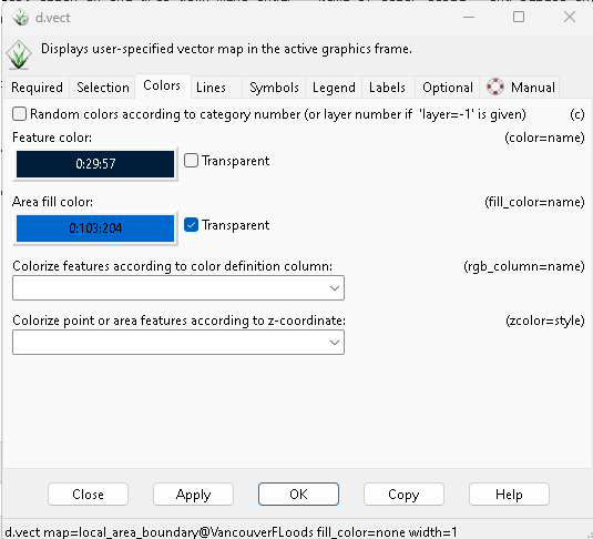
: 5. Under the '''Colors''' tab, select a color for the boundary itself and check ''Transparent'' for the ''Area fill color'', and click on '''OK''' |
|||
: - To better visualize the elevation of the study area we will set the transparency of the boundary area fill colour to transparent |
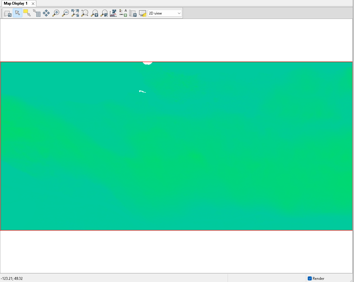
|||
[[File:Propertiess.PNG]] |
|||
: '''1.''' Right click on the "local-area-boundary" layer in the "Layer" panel |
|||
: '''2.''' Select layer properties and navigate to the "colours" tab |
|||
: '''3.''' Select the transparent option for the "Area fill colour" |
|||
[[File:VectColour.png|frame|left|Changing the transparency of vector layer]] |
|||
<div style="clear: left;"></div> |
|||
===Determining Approximate Low-Point=== |
|||
: - We have our map ready to run a basic flood risk assessment using the raster calculator |
|||
: - But first, we need to determine the lowest approximate elevation according to our Vancouver DEM |
|||
: - To do so, we will make use of the visual query tool at the top of the map viewer |
|||
[[File:Query.png|frame|left|The visual query tool]] |
|||
: '''1.''' The first step in determining an approximate "lowest point" in the DEM is using prior knowledge to predict where the lowest elevation point may occur. In this tutorial we assume the low points will occur near the coastal edge of Vancouver |
|||
: '''2.''' Now that we have defined where to look to find the approximate "lowest point" we will use the query tool to sample along the shoreline to determine the lowest elevation value (the values will be associated with a colour and when query will return a pixel value [m]) |
|||
[[File:QueryDetermine.png|frame|center|An example of the returned values of the query toll]] |
|||
: '''3.''' Finally we can determine that the lowest points of our DEM are at sea level or 0 m. Although our boundary falls on the 0 m zone in the DEM it is unlikely that there is any notable development along that range and for the purpose of this tutorial will be considered shoreline. |
|||
===Creating Flooding Scenarios=== |
|||
: '''1.''' Under the '''Raster''' tab, navigate to the "Raster map calculator" drop-down and select "Raster map calculator" [r.mapcalc], not to be confused with the simple raster calculator |
|||
: '''2.''' Input this expression to simulate water levels of 6m: VancouverFlood6m = '''( ( VancouverDEM@VancouverFLoods <= 6 ) == 1 ) & ( ( VancouverDEM@VancouverFLoods >= 6 ) == 0 ) *supplement VancouverDEM with whatever you named the ''SRTM DEM'' file* |
|||
: '''Note''' @VancouverFLoods is the name of the current mapset |
|||
: '''3.''' Click on '''Run''' |
|||
: '''Before Simulated Flooding ''' |
|||
[[File:BeforeFloods.png|frame|center|Vancouver BC before simulated flooding]] |
|||
:'''After Simulated Flooding''' |
|||
[[File:AfterFloods.png|frame|center|The simulated result of 6 meter flood waters in Vancouver BC]] |
|||
: - The resultant raster map shows which areas are inundated (yellow) and the non-inundated areas (purple) at 6 meters of flood water. Looking closer at the results, we can see that in comparison to our previous map the raster cell values which varied and corresponded to elevation values, now corresponds to regions affected and unaffected by flood waters on a binary scale 1 meaning flood water and 0 meaning dry land. |
|||
: - Next let's simulate the effects of 9 meters of flood water to see if there is any significant difference in impact. |
|||
: '''1.''' Under the '''Raster''' tab, select '''Raster map calculator''' [r.mapcalc] |
|||
: '''2.''' Input this expression to simulate water levels of 9m: VancouverFlood9m = '''( ( VancouverDEM@VancouverFLoods <= 9 ) == 1 ) & ( ( VancouverDEM@VancouverFLoods >= 9 ) == 0 )''' *supplement VancouverDEM with whatever you named the ''SRTM DEM'' file* |
|||
: '''3.''' Click on '''Run''' |
|||
:'''Simulated Flooding of 9 Meters''' |
|||
[[File:9mFLood.png|frame|center|The simulated result of 9 meter flood waters in Vancouver BC]] |
|||
: - It is clear the resulting Raster is representing a similar relationship to the last, but now symbolizing 9 meters rather than 6 meters. Finally, we will demonstrate a severe case of flooding at 20 meter flood waters. |
|||
: - Modify the existing equation to simulate 20 meter flood waters: VancouverFlood20m = '''( ( VancouverDEM@VancouverFLoods <= 20 ) == 1 ) & ( ( VancouverDEM@VancouverFLoods >= 20 ) == 0 )''' |
|||
[[File:Basemap.PNG]] |
|||
[[File:Severeflooding.png|frame|center|The simulated result of 20 meter flood waters in Vancouver BC]] |
|||
===Creating flooding scenarios=== |
|||
We have our map ready to run a basic flood risk assessment using the raster calculator. The lowest points of elevation in Daytona Beach is approximately 4m, but we will simulate an initial rise of 2m to conservatively determine the effects of flooding. |
|||
: 1. Under the '''Raster''' tab, select '''Raster map calculator''' [r.mapcalc] |
|||
: 2. Input this expression to simulate water levels of 6m: DaytonaFLOOD2m = '''( ( DaytonaSRTM@PERMANENT <= 6 ) == 1 ) & ( ( DaytonaSRTM@PERMANENT >= 6 ) == 0 ) *supplement DaytonaSRTM with whatever you named the ''SRTM DEM'' file* |
|||
: 3. Click on '''Run''', make sure the ''Add created raster map into layer tree'' option is selected before doing so |
|||
[[File:Flood2m.PNG]] |
|||
: - The results clearly display the more ravaging effects on infrastructure and subsequently people with the simulated severe case of flooding. |
|||
The resultant raster map shows which areas are inundated (yellow) and the non-inundated areas (purple) at 2m sea level rise. Next we will create another raster map showing an example of 5m of rising sea level. |
|||
: 1. Under the '''Raster''' tab, select '''Raster map calculator''' [r.mapcalc] |
|||
: 2. Input this expression to simulate water levels of 6m: DaytonaFLOOD2m = '''( ( DaytonaSRTM@PERMANENT <= 9 ) == 1 ) & ( ( DaytonaSRTM@PERMANENT >= 9 ) == 0 ) *supplement DaytonaSRTM with whatever you named the ''SRTM DEM'' file* |
|||
: 3. Click on '''Run''', make sure the ''Add created raster map into layer tree'' option is selected before doing so |
|||
[[File:Flood5m.png]] |
|||
== |
==Conclusion== |
||
: - After having created 3 separate raster layers, representing (although crudely) 6 meter flooding, 9 meter flooding and 20 meter flooding respectively, we can complete our assessment by toggling the layers on and off in the panel to contrast the differences in impact of each flood level. |
|||
By toggling between the original ''SRTM DEM'', ''2m Flooding'', and ''5m Flooding layers'', we can ascertain the levels of flooding we could see in areas in and around Daytona Beach. |
|||
: - Although this was just a basic assessment of flood levels conducted on GRASS GIS, the fundamentals of this tutorial are re-applicable to much more in depth analysis and have effectively equipped you with the knowledge and resources to expand to much higher level results. |
|||
: - Different types of data that could/should be incorporated to simulating flood levels in your locality may include: Precipitation data, Land cover data, Slope and Aspect (which can be derived from the DEM using raster tools!). |
|||
Latest revision as of 17:46, 29 September 2023
Contents
Introduction
With the prevalence of climate change in society today many individuals are discovering the advantageous functionality of Geographic Information Systems (GIS) for modelling and predicting the ramifications of climate change to their localities. The climate crisis brings about many pressing issues to the world, but this tutorial will prioritize emulating rising water levels to demonstrate a very basic flood risk assessment using open source software and data. This tutorial will make use of GRASS GIS to demonstrate the recently updated user-friendly Graphical User Interface and will focus on conducting a basic flood risk analysis on one of Canada's most populated coastal cities, Vancouver BC. This tutorial uses open source data from USGS's Earth Explorer and the City of Vancouver's Open Data website.
Vancouver is one of Canada's largest coastal cities and experiences the ramifications of climate change much more severely than us at Carleton University in Ottawa. An article by CBC ([1]) provides some context to the tutorial with recent (as of 2022) flooding in the city to emphasize the importance as well as the potential that GIS holds in aiding communities at a national scale.
Software and Data
This tutorial uses the latest version of Grass GIS 8.3.0, which can be downloaded for Windows, MacOSX, and Linux from their website ([2]). After downloading, run the installer and install GRASS onto your computer. Ensure to download it to a secure directory with a known location so you can easily keep track of things. The installer will most likely prompt you to install the Microsoft Visual C++ Redistributable; allow this install as it is integral for the GRASS GIS runtime. This tutorial aims to focus on using the updated GUI but will brush on the command console and its ease of use in GRASS.
The data used for this lesson are derived from two main sources, the US Geological Survey Earth Explorer tool ([3]) and the City of Vancouver Open Data website ([4]); both are open data sources, although the USGS requires you to create an account to access their data.
Vancouver Open Data
First, let's begin by collecting the data needed from the City of Vancouver Open Data Website:
- 1. Open the link provided above
- 2. Select the Catalogue tab in the left of the home page
- 3. A catalogue browser will open, in the search bar enter "Local Area Boundary"
- 4. Select the file containing the cities 22 planning areas (this will serve as our city boundary)
- 5. Inspect the integrity of the data by reviewing the metadata, paying specific attention to the Data Accuracy, Last Processed Date and the Data Owner
- 6: Select the "Export" tab and select the hyperlink for the Shapefile download
- 7: Repeat this process for another Shapefile called "Public Streets"
- 8. Store the data in a folder you'll keep tabs on (we will export it to the GRASS database later)
USGS Earth Explorer
Next, we will collect the data from the Earth Explorer website:
- 1. Open the link provided from above
- 2. Select the Data Sets tab at the top of the window
- 3. Expand the Digital Elevation menu, expand the SRTM submenu, select SRTM 1 Arc-Second Global
- 4. Return to the Search Criteria tab
- 5. Under the "Select a Geocoding Method" drop down tab select Address/Place and enter Vancouver
- 6. Select the coordinates for Vancouver BC and click the "Results" tab
- 7. Under results a DEM should appear, start by inspecting the metadata
- 8. First click "Show Footprint" to ensure the image covers the study area
- 9. Next click "Show metadata" and browse, paying close attention to acquisition date and Resolution to determine the units and accuracy of the data
- 10. Finally click "Download Options" and select "TIFF" format; store the resulting TIFF file somewhere safe for now
Exploring the GRASS GUI
Starting a GRASS session
- Now that GRASS is properly installed, and our data has been collected and inspected, we can continue with starting a GRASS session. A reminder that the software for this tutorial is 8.3.0; a benefit to open source software, like GRASS, isthat previous software releases are still available for public use if you find need for following an older tutorial.
- Let us being by creating a GRASS session:
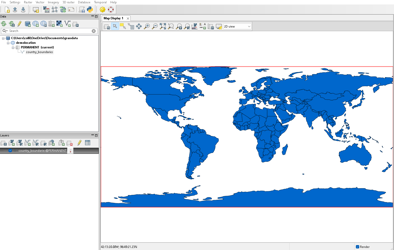
- First, open Grass GIS by clicking on the desktop icon; if your installer did not create a desktop shortcut manually search for the GRASS GIS app in your operating system's search bar
- Next, you will see (any returning users will be shocked) that the GRASS GUI loads an automatic "demolocation")
- Notice:
- On the left hand side, under the pane titled "Data", GRASS GIS has loaded a "demolocation" as well as a "PERMANENT" mapset
- This is a new feature of GRASS GIS and provides a much more user friendly experience for learning the storage method used by GRASS
- This tutorial will briefly outline the basics behind the GRASS storage system while walking you through the simple GUI
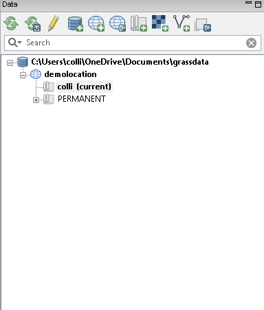
The Data Panel
- Notice: On the left hand side of the GUI there is a data panel as mentioned above
- - This panel allows the user to control a few factors:
- 1. The GRASS Database: This allows the user to add new/existing databases and remove them as well
- 2. The project's location: This feature allows the user to specify a location which is essentially a sub-directory in the database
- 3. Creating a Mapset: This allows the user to create a new map workspace much like the already created "PERMANENT" mapset
- - The other two icons in the data panel will be made of later when importing our data.
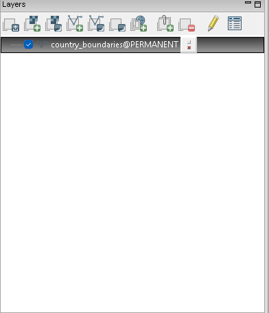
The Layers Panel
- Notice: To the left is an image of the layers panel
- - The layers panel includes a few more tools than the Data panel and may come across as intimidating to beginners but is quite simple for our application
- - The layers panel allows users to view the loaded layers in the Map Display, as well as gives users the tools to add or create a user defined raster/vector layer or map
- - There is an option to add a service layer (WMS, WMTS, NASA OnEarth) which are map layers online
- - For the purpose of this tutorial we will focus on the layers that are currently displayed in our map display, and in this current instance that is the "country_boundaries" layer loaded in the mapset "PERMANENT" (represented by @PERMANENT)
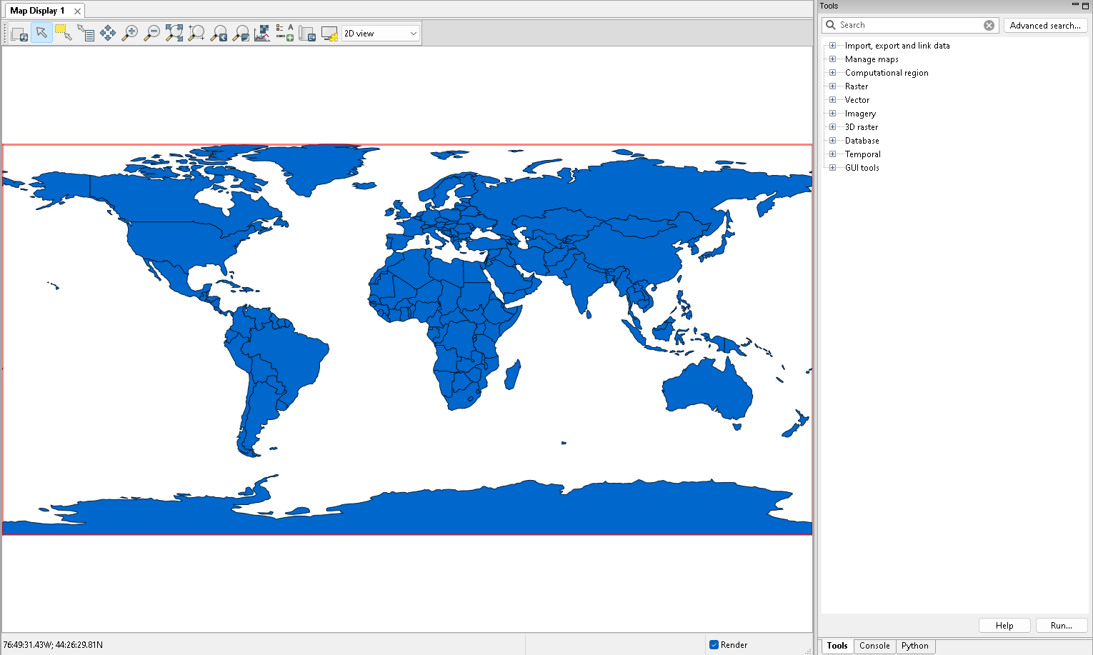
The Map Display and Tools Panel
- Notice: Above is the "Map Viewer" and "Tools" panel
- - Finally the map viewer and tools panel are the last two components of the GUI to address with the remainder of the applications found at the top of the GUI
- - The map viewer is a basic view of the loaded layers in the mapset and multiple viewers can be opened at once under File and Map display
- - The tools panel is home to all of the potential GIS operational tools
- - Since this software is open source all of these tools are available to all users, and are also accessible in a development environment without even loading the GUI!
Methods
Setting Up the Workspace
- - The firs step in conducting a flood risk assessment is establishing the correct database, location and mapset for the study area
- - After establishing a proper workspace, we can set a computational region for the study area, so that the GIS understands our location of interest
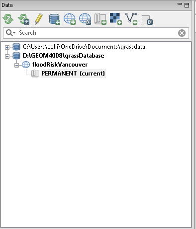
- 1. Create a new database in the data panel
- - Clicking this tool will open a file explorer window and prompt you to either find a location where an existing database resides, or you can create a new file in a trusted directory to act as your new GRASS database. We will choose the latter
- - Create a database in the directory of your choosing and title it "grassDatabase" as a general location to store our GRASS data
- - The result is a new, empty database
- - Following the creation of the database GRASS will prompt the user asking if they'd like to create a new location
- - Select yes and being creating a new location (if the prompt does not show, use the manual tool in the data panel)
- 2. Create a new location
- - Enter a meaningful name for the location such as "floodRiskVancouver"
- - Be sure to change the database directory from the default to the created database
- - Select the WGS 84 / UTM zone 10N EPSG as that is the UTM zone for Vancouver
- - The result will be the creation of the new location as seen in the data panel as well as a new PERMANENT mapset for that location
- 3. Create a new mapset/set region
- - Enter an appropriate name for the "fresh" mapset
- - Provide the mapset with a meaningful name
- - Finally, under the "Settings" drop-down tab select "Computational Region"
- - Select set region [g.region], and once the panel prompt appears, select "Set Region to Match Vector Map" and select the boundary file
- - As mentioned before this defines the area of interest so that when we import our raster file, it only displays what falls in the region (removing the need for [r.clip] in smaller projects which is now an add-on available in the extensions)
- - Now we are ready to conduct our assessment!
Importing Vector Data into GRASS
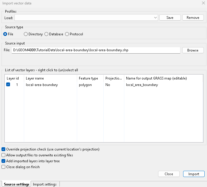
The GRASS session is now setup, and we can start importing the data we collected from earlier, starting with the local area boundary file
- 1. Either under the File tab or the Data panel, select the "Import Vector Data" tool [v.import]
- 2. Browse to the location you selected to extract our data and select the "local-area-boundary" Shapefile
- 3. Ensure the Override Projection Check is selected allowing whatever projection our data is currently projected in (if projected at all) to be projected in the same format as the location we created
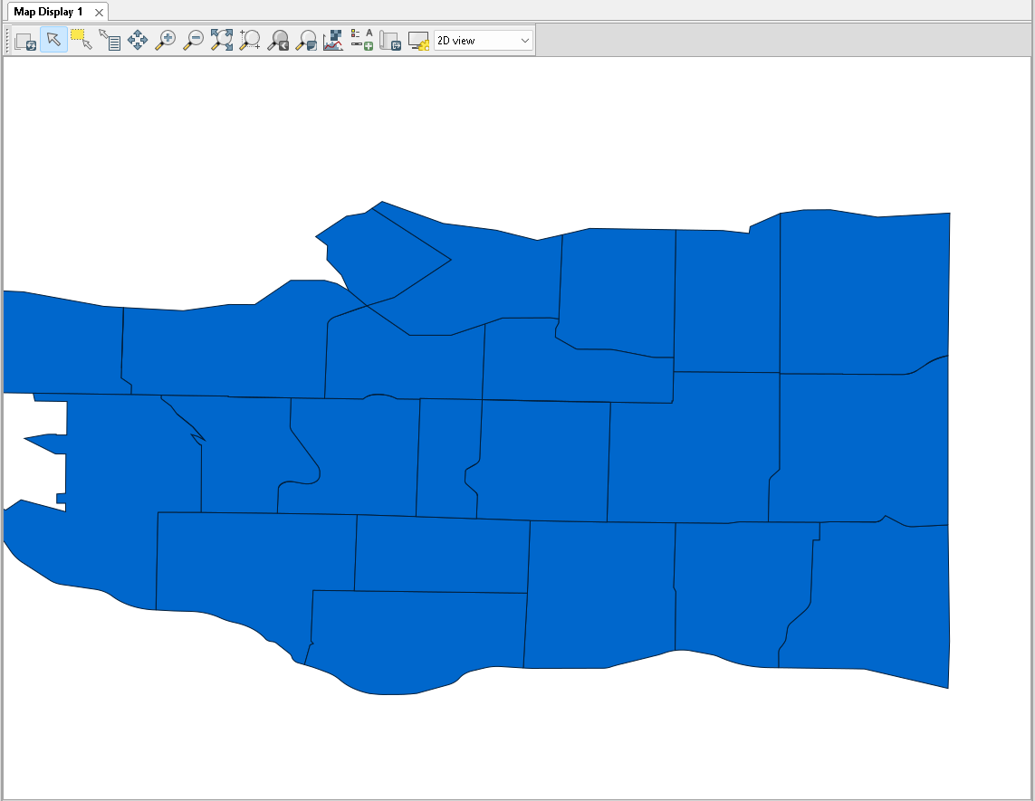
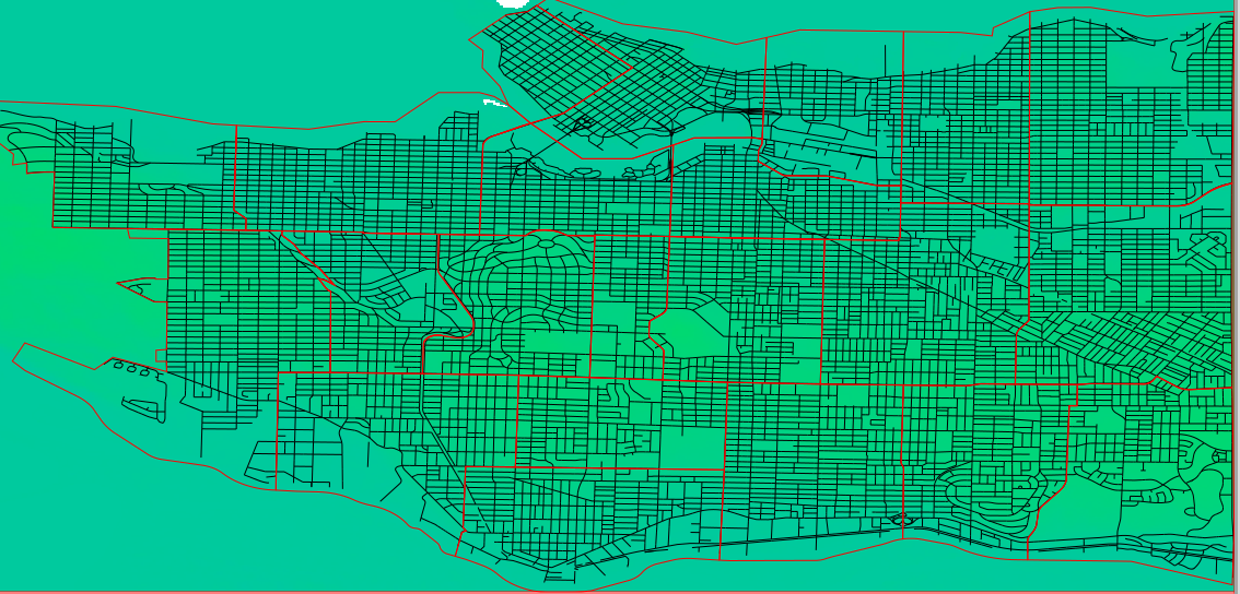
- - The result should be the Vancouver boundary layer displayed in the map viewer:
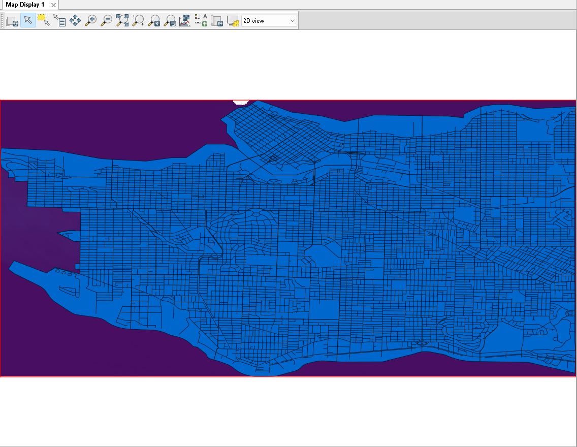
- - Finally, we will import the "Public-streets" Shapefile following the same process
Importing Raster Data into GRASS
Now we can import the SRTM (Shuttle Radar Topography Mission [[5]] DEM (Digital Elevation Model) we downloaded earlier from the USGS Earth Explorer:
- 1. Under the File or Data Panel select import raster data [r.import]
- 2. Browse to the location of the SRTM DEM
- 3. Select Override projection check and select import
Changing Raster Symbology
Now that we have the data displayed, we can adjust the symbology to better suit our applications:
- 1. Right-click on the SRTM DEM layer and select Set color table
- 2. Ensure that the correct raster file is selected
- 3. Under the Define tab, click on the drop-down menu under Name of color table and select the elevation color table, and click on Run
Changing Vector Symbology
- - To better visualize the elevation of the study area we will set the transparency of the boundary area fill colour to transparent
- 1. Right click on the "local-area-boundary" layer in the "Layer" panel
- 2. Select layer properties and navigate to the "colours" tab
- 3. Select the transparent option for the "Area fill colour"
Determining Approximate Low-Point
- - We have our map ready to run a basic flood risk assessment using the raster calculator
- - But first, we need to determine the lowest approximate elevation according to our Vancouver DEM
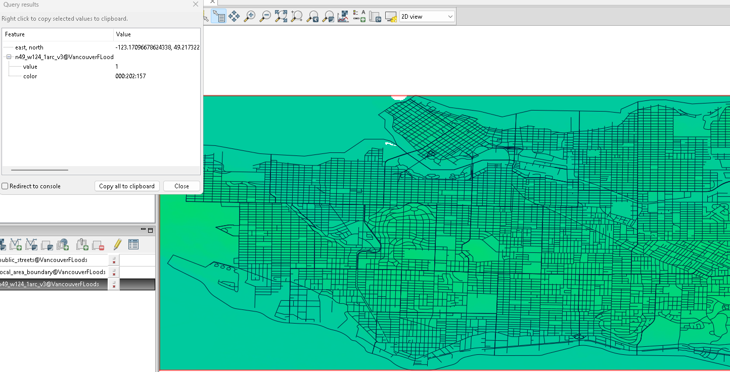
- - To do so, we will make use of the visual query tool at the top of the map viewer
- 1. The first step in determining an approximate "lowest point" in the DEM is using prior knowledge to predict where the lowest elevation point may occur. In this tutorial we assume the low points will occur near the coastal edge of Vancouver
- 2. Now that we have defined where to look to find the approximate "lowest point" we will use the query tool to sample along the shoreline to determine the lowest elevation value (the values will be associated with a colour and when query will return a pixel value [m])
- 3. Finally we can determine that the lowest points of our DEM are at sea level or 0 m. Although our boundary falls on the 0 m zone in the DEM it is unlikely that there is any notable development along that range and for the purpose of this tutorial will be considered shoreline.
Creating Flooding Scenarios
- 1. Under the Raster tab, navigate to the "Raster map calculator" drop-down and select "Raster map calculator" [r.mapcalc], not to be confused with the simple raster calculator
- 2. Input this expression to simulate water levels of 6m: VancouverFlood6m = ( ( VancouverDEM@VancouverFLoods <= 6 ) == 1 ) & ( ( VancouverDEM@VancouverFLoods >= 6 ) == 0 ) *supplement VancouverDEM with whatever you named the SRTM DEM file*
- Note @VancouverFLoods is the name of the current mapset
- 3. Click on Run
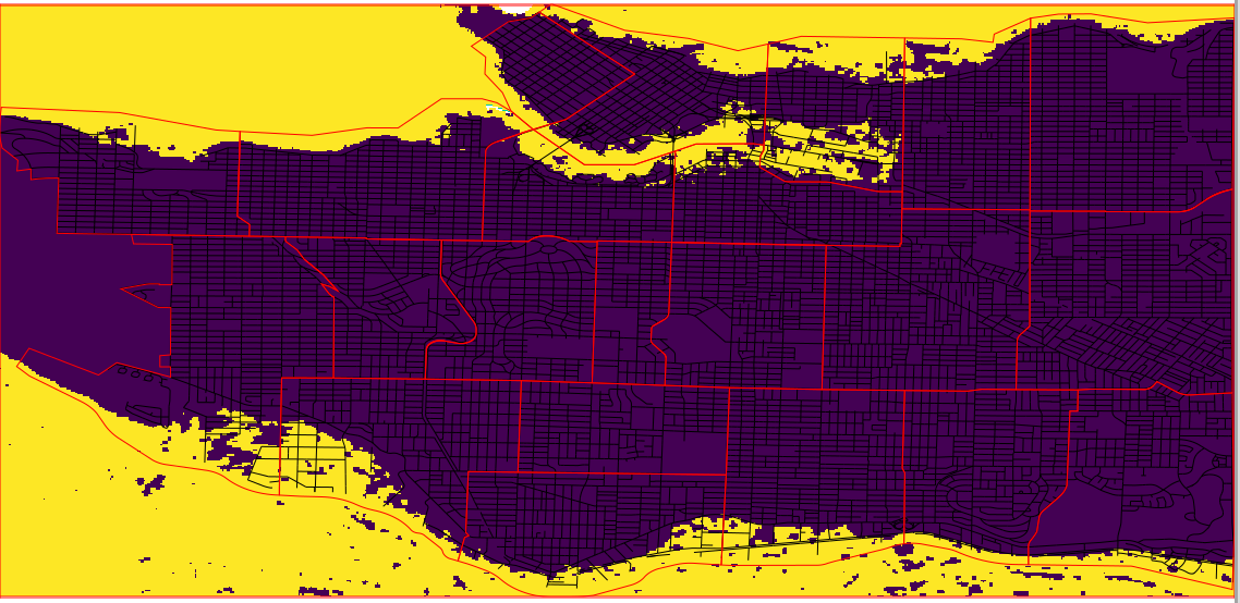
- Before Simulated Flooding
- After Simulated Flooding
- - The resultant raster map shows which areas are inundated (yellow) and the non-inundated areas (purple) at 6 meters of flood water. Looking closer at the results, we can see that in comparison to our previous map the raster cell values which varied and corresponded to elevation values, now corresponds to regions affected and unaffected by flood waters on a binary scale 1 meaning flood water and 0 meaning dry land.
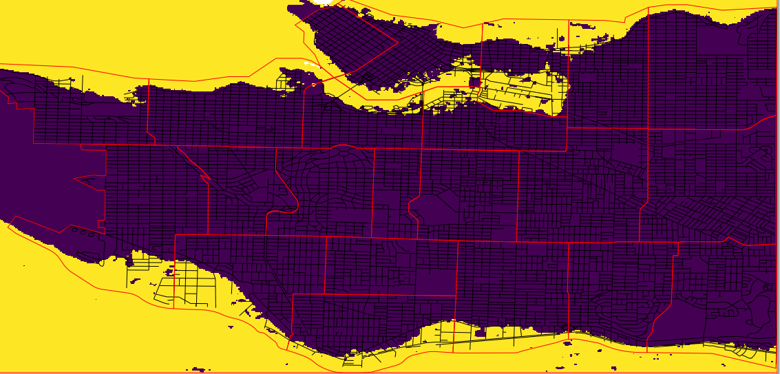
- - Next let's simulate the effects of 9 meters of flood water to see if there is any significant difference in impact.
- 1. Under the Raster tab, select Raster map calculator [r.mapcalc]
- 2. Input this expression to simulate water levels of 9m: VancouverFlood9m = ( ( VancouverDEM@VancouverFLoods <= 9 ) == 1 ) & ( ( VancouverDEM@VancouverFLoods >= 9 ) == 0 ) *supplement VancouverDEM with whatever you named the SRTM DEM file*
- 3. Click on Run
- Simulated Flooding of 9 Meters
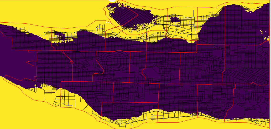
- - It is clear the resulting Raster is representing a similar relationship to the last, but now symbolizing 9 meters rather than 6 meters. Finally, we will demonstrate a severe case of flooding at 20 meter flood waters.
- - Modify the existing equation to simulate 20 meter flood waters: VancouverFlood20m = ( ( VancouverDEM@VancouverFLoods <= 20 ) == 1 ) & ( ( VancouverDEM@VancouverFLoods >= 20 ) == 0 )
- - The results clearly display the more ravaging effects on infrastructure and subsequently people with the simulated severe case of flooding.
Conclusion
- - After having created 3 separate raster layers, representing (although crudely) 6 meter flooding, 9 meter flooding and 20 meter flooding respectively, we can complete our assessment by toggling the layers on and off in the panel to contrast the differences in impact of each flood level.
- - Although this was just a basic assessment of flood levels conducted on GRASS GIS, the fundamentals of this tutorial are re-applicable to much more in depth analysis and have effectively equipped you with the knowledge and resources to expand to much higher level results.
- - Different types of data that could/should be incorporated to simulating flood levels in your locality may include: Precipitation data, Land cover data, Slope and Aspect (which can be derived from the DEM using raster tools!).
