Difference between revisions of "Path Analysis with Vector Data Using QGIS"
(→Data) |
|||
| (39 intermediate revisions by 2 users not shown) | |||
| Line 1: | Line 1: | ||
== '''Introduction''' == |
== '''Introduction''' == |
||
QGIS is an application that is used for GIS (Geographic Information Systems) purposes that is Free and Open Source Software (FOSS). This software is user friendly. It runs on Linux, Unix, Windows, Mac OSX and Android. QGIS supports a variety of raster, vector and database formats and functions. It provides a |
QGIS is an application that is used for GIS (Geographic Information Systems) purposes that is Free and Open Source Software (FOSS). This software is user friendly. It runs on Linux, Unix, Windows, Mac OSX and Android. QGIS supports a variety of raster, vector and database formats and functions. It provides a continuously growing number of capabilities, provided by core functions and plugins. With QGIS, the user can manage, edit, conduct data analysis, visualize and create maps. |
||
| Line 9: | Line 9: | ||
This tutorial will guide the user through the process of downloading data, adding it to QGIS and conducting the analysis to find sections on a trail that connect to other path networks. In this tutorial, we will combine a variety of path networks and will find ways to access the main trail through these networks. |
This tutorial will guide the user through the process of downloading data, adding it to QGIS, and conducting the analysis to find sections on a trail that connect to other path networks. In this tutorial, we will combine a variety of path networks and will find ways to access the main trail through these networks. Using the intersections between the main trail and the other pathway networks, we will find the shortest distances possible to get from any location in the city to the main trail. This tutorial has two goals: (1) to find ways to access the main trail from different areas within the city, and (2)to identify the paths of shortest distance from any location to all of the main trail intersections. This type of analysis can be used for any type of path analysis and is applicable to other data sets. We will use the Rideau Trail as the main trail that we are analyzing. The other paths that we will be using to access the Rideau Trail are city roads, cycling routes, paths and parks. The data that are used here are all open data. This tutorial is intended for beginners, it is assumed that the user does not have any GIS knowledge. |
||
== '''Objective''' == |
== '''Objective''' == |
||
In the [[Path_Analysis_with_Vector_Data_Using_QGIS#Process|Process]] section of this tutorial, we will be conducting an analysis of data on The Rideau Trail, in combination with other trail, path, and road data. To access The Rideau Trail, we will need to find which lines intersect with it. The process demonstrated in this tutorial will allow us to find which paths or roads within Ottawa intersect with The Rideau Trail, to highlight potential access points in different sections of the city. |
|||
The Rideau Trail is a hiking trail that links Ottawa to Kingston, 387 km long. The Rideau Trail Association maintains the trail |
The Rideau Trail is a hiking trail that links Ottawa to Kingston, 387 km long. The Rideau Trail Association maintains the trail and also provides additional information so others can use it to it’s full potential. Once we have conducted our analysis, we will cross reference our information with maps provided by the Rideau Trail Association. The map keys will help us identify which maps we will need to view the area in more detail. |
||
In the [[Path_Analysis_with_Vector_Data_Using_QGIS#Shortest_Path_Analysis|Shortest Path Analysis]] section of this tutorial, we will be using the various pathway intersections to find ways to access The Rideau Trail from different areas within the city, and to identify the paths of shortest distance from any location to one of the main trail intersections. |
|||
== '''Data''' == |
== '''Data''' == |
||
The type of data that we will be using are Keyhole Markup Language (KML) and shapefiles. We will be using vector data for this analysis (spatial data which represents features using points, lines, or polygons). KML is a file format that is used to |
The type of data that we will be using are Keyhole Markup Language (KML) and shapefiles. We will be using vector data for this analysis (spatial data which represents features using points, lines, or polygons). KML is a file format that is used to hold geographic data. It is an international standard that is maintained by the Open Geospatial Consortium, Inc. (OGC). A shapefile is another data format used by GIS software to hold geospatial vector data and despite the name, it actually consists of three or more files, all with the same prefix filename but different extensions (.shp, .shx, .dbf, ...). |
||
The data that will be used for this tutorial can be found from the following links: |
The data that will be used for this tutorial can be found from the following links: |
||
Cycling_Network: https://open.ottawa.ca/datasets/cycling-network |
Cycling_Network: https://open.ottawa.ca/datasets/cycling-network (Download shapefile) |
||
| ⚫ | |||
| ⚫ | |||
Park_Paths: https://open.ottawa.ca/datasets/park-paths |
|||
Park_Paths: https://open.ottawa.ca/datasets/park-paths (Download shapefile) |
|||
Road_Centrelines: https://open.ottawa.ca/datasets/road-centrelines (Download shapefile) |
|||
| ⚫ | |||
| ⚫ | |||
== '''Process'''== |
== '''Process'''== |
||
| Line 45: | Line 46: | ||
Add the data that will be used. |
Add the data that will be used. First, you must unzip the newly downloaded files and save them to a desirable working directory. To add the data, use the Browser panel that appears on the left-hand side of QGIS, as seen in Figure 2. If you do not see the Browser panel, enable it by clicking View > Panels > Browser. Using the Browser panel, navigate to the file folder that you have saved the downloaded data sets in. Once you have found your data, you can double-click it in the Browser panel to add it into the QGIS project. Alternatively, you can also drag-and-drop the data from the Browser panel into the Layers panel as well. The data will be unorganized. You can turn off the map keys layer. It will be used for a later purpose, to cross-reference with other maps. |
||
We will now conduct the path analysis of intersections to the main trail. Click the tab Vector |
We will now conduct the path analysis of intersections to the main trail. Click the tab Vector > Analysis Tools > Line intersections... |
||
| Line 82: | Line 83: | ||
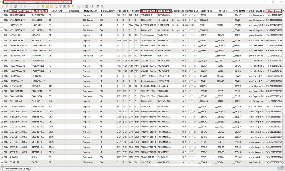
'''Figure 7.''' An opened attribute table for the layer ''Road_Centrelines_Intersections''. In this attribute table, geographic information such as road name in which the intersection point is located on, name of accessing roads and length of road. This information can be useful when planning a trip. |
'''Figure 7.''' An opened attribute table for the layer ''Road_Centrelines_Intersections''. In this attribute table, geographic information such as road name in which the intersection point is located on, name of accessing roads and length of road. This information can be useful when planning a trip. |
||
| ⚫ | |||
== '''Cross-Referencing With Other Maps''' == |
== '''Cross-Referencing With Other Maps''' == |
||
| Line 118: | Line 118: | ||
'''Figure 11.''' The same data that was used in the previous analysis can be read in ''Google Earth Pro''. |
'''Figure 11.''' The same data that was used in the previous analysis can be read in ''Google Earth Pro''. |
||
== '''Shortest Path Analysis''' == |
|||
Using the intersections layers created in the [[Path_Analysis_with_Vector_Data_Using_QGIS#Process|Process]] section, we will now use a Network Analysis tool within QGIS to calculate the shortest path between any random point in Ottawa and the intersection points of The Rideau Trail. Say you wanted to access The Rideau Trail from Carleton Universtiy, but you only wanted to travel along the roads to get to it. In this scenario, we will be using the Roads_Centrelines layer and the Roads_Centreline_Intersections points that were previously created to find the shortest distances possible to each of the places where a road and The Rideau Trail intersect. This analysis aims to answer the question, how do I get to the Rideau Trail using roads from my location in Ottawa? |
|||
NOTE: This analysis was conducted using QGIS 3.4. |
|||
[[File:Figure_12..png|caption|border|1000px]] |
|||
'''Figure 12.''' Start by having your Road_Centrelines_Intersections, Road_Centrelines, Main Trail, and Ottawa_Neighbourhoods layers turned on with easy to view symbology. |
|||
Next, open the QGIS toolbox by clicking the gear icon on the Attributes toolbar. If you cannot find this icon, go to Processing > Toolbox. |
|||
[[File:Figure13 MM.png|caption|border|1000px|]] |
|||
'''Figure 13.''' The location of the Toolbox icon on the Attributes toolbar. |
|||
After clicking the Toolbox, click on the drop-down menu beside Network analysis. There will be several options, but click on the Shortest path (point to layer) tool. The Shortest path (point to layer) tool is an algorithm that calculates the shortest path between a given start point and multiple end points using a vector layer. |
|||
[[File:Figure14 MM.png|caption|border|1000px]] |
|||
'''Figure 14.''' The location of the Shortest path (point to layer) tool in the Network analysis toolbox. |
|||
Clicking on the Shortest path (point to layer) tool will bring up a separate window. In the Parameters window, the ''Vector layer representing network'' will be the Road_Centrelines layer. The ''Path type to calculate'' will be Shortest. The ''Vector layer with end points'' will be the Roads_Centerlines_Intersections layer. |
|||
[[File:Figure15 MM.png|caption|border|500px]] |
|||
'''Figure 15.''' The desired configuration in the parameters window. |
|||
Before hitting ''Run'', you will have to select a starting point for the algorithm to calculate the shortest distance. In the parameters window, click on the ''Start point (x, y)''. This will minimize the window to your map view, and your cursor will be a cross hair. Select an area on Carleton University's campus. |
|||
[[File:Figure16 MM.png|caption|border|1000px]] |
|||
'''Figure 16.''' Selecting a desired start point on Carleton University's campus. |
|||
Once you have selected a starting point, the Shortest path (point to layer) window will maximize, and you may now hit the ''Run'' function in the bottom right corner of the window. Running this tool will create a temporary layer, and will demonstrate all the different shortest pathway possibilities to get to any of the locations where the road intersects The Rideau Trail as if you were travelling by the Roads_Centrelines layer. |
|||
[[File:Figure17 MM.png|caption|border|1000px]] |
|||
'''Figure 17.''' A screenshot of the layer created by the Shortest path (point to layer) tool. This layer displays all of the shortest pathways from the chosen start point at Carleton University to each location where the Road_Centrelines layer intersects the Main Trail (Rideau Trail). |
|||
Opening up the attribute table of the new Shortest path layer will reveal several attribute columns, however, the columns of most interest include the start and cost columns. The start and cost columns represent the distance between the start point (start) and the end point (cost) in layer units. In this case, the start and the cost are represented in latitude and longitude coordinates. If interested, you can use these coordinates to calculate the exact distance between each start and end point. |
|||
[[File:Figure18 MM.png|caption|border|500px]] |
|||
| ⚫ | |||
'''Figure 18.''' The start and cost columns in the attribute table of the Shortest path layer. |
|||
This analysis can be completed using any of the other path network and intersection layers as well. |
|||
== '''References''' == |
== '''References''' == |
||
ESRI. (1998). ''ESRI Shapefile Technical Description'' (PDF). Retrieved from https://www.esri.com/library/whitepapers/pdfs/shapefile.pdf |
|||
Google Developers. (2019). ''Keyhole Markup Language''. Retrieved from https://developers.google.com/kml |
Google Developers. (2019). ''Keyhole Markup Language''. Retrieved from https://developers.google.com/kml |
||
Latest revision as of 12:16, 19 October 2020
Contents
Introduction
QGIS is an application that is used for GIS (Geographic Information Systems) purposes that is Free and Open Source Software (FOSS). This software is user friendly. It runs on Linux, Unix, Windows, Mac OSX and Android. QGIS supports a variety of raster, vector and database formats and functions. It provides a continuously growing number of capabilities, provided by core functions and plugins. With QGIS, the user can manage, edit, conduct data analysis, visualize and create maps.
Figure 1. The latest release is QGIS 3.10 at the time of this writing; see qgis.org.
This tutorial will guide the user through the process of downloading data, adding it to QGIS, and conducting the analysis to find sections on a trail that connect to other path networks. In this tutorial, we will combine a variety of path networks and will find ways to access the main trail through these networks. Using the intersections between the main trail and the other pathway networks, we will find the shortest distances possible to get from any location in the city to the main trail. This tutorial has two goals: (1) to find ways to access the main trail from different areas within the city, and (2)to identify the paths of shortest distance from any location to all of the main trail intersections. This type of analysis can be used for any type of path analysis and is applicable to other data sets. We will use the Rideau Trail as the main trail that we are analyzing. The other paths that we will be using to access the Rideau Trail are city roads, cycling routes, paths and parks. The data that are used here are all open data. This tutorial is intended for beginners, it is assumed that the user does not have any GIS knowledge.
Objective
In the Process section of this tutorial, we will be conducting an analysis of data on The Rideau Trail, in combination with other trail, path, and road data. To access The Rideau Trail, we will need to find which lines intersect with it. The process demonstrated in this tutorial will allow us to find which paths or roads within Ottawa intersect with The Rideau Trail, to highlight potential access points in different sections of the city.
The Rideau Trail is a hiking trail that links Ottawa to Kingston, 387 km long. The Rideau Trail Association maintains the trail and also provides additional information so others can use it to it’s full potential. Once we have conducted our analysis, we will cross reference our information with maps provided by the Rideau Trail Association. The map keys will help us identify which maps we will need to view the area in more detail.
In the Shortest Path Analysis section of this tutorial, we will be using the various pathway intersections to find ways to access The Rideau Trail from different areas within the city, and to identify the paths of shortest distance from any location to one of the main trail intersections.
Data
The type of data that we will be using are Keyhole Markup Language (KML) and shapefiles. We will be using vector data for this analysis (spatial data which represents features using points, lines, or polygons). KML is a file format that is used to hold geographic data. It is an international standard that is maintained by the Open Geospatial Consortium, Inc. (OGC). A shapefile is another data format used by GIS software to hold geospatial vector data and despite the name, it actually consists of three or more files, all with the same prefix filename but different extensions (.shp, .shx, .dbf, ...).
The data that will be used for this tutorial can be found from the following links:
Cycling_Network: https://open.ottawa.ca/datasets/cycling-network (Download shapefile)
Ottawa_Neighbourhood_Study_ONS_Neighbourhood_Boundaries_Gen_2: https://open.ottawa.ca/datasets/ottawa-neighbourhood-study-ons-neighbourhood-boundaries-gen-2 (Download shapefile)
Park_Paths: https://open.ottawa.ca/datasets/park-paths (Download shapefile)
Road_Centrelines: https://open.ottawa.ca/datasets/road-centrelines (Download shapefile)
Rideau Trail: https://www.rideautrail.org/discover-the-trail/maps/ (Download KML file)
Process
Please download the data from the previous section before starting the tutorial.
Open QGIS 3.10.
Figure 2. Open a new project and give it a name.
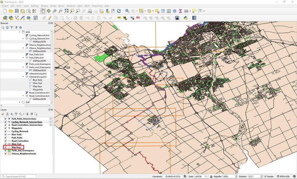
Add the data that will be used. First, you must unzip the newly downloaded files and save them to a desirable working directory. To add the data, use the Browser panel that appears on the left-hand side of QGIS, as seen in Figure 2. If you do not see the Browser panel, enable it by clicking View > Panels > Browser. Using the Browser panel, navigate to the file folder that you have saved the downloaded data sets in. Once you have found your data, you can double-click it in the Browser panel to add it into the QGIS project. Alternatively, you can also drag-and-drop the data from the Browser panel into the Layers panel as well. The data will be unorganized. You can turn off the map keys layer. It will be used for a later purpose, to cross-reference with other maps.
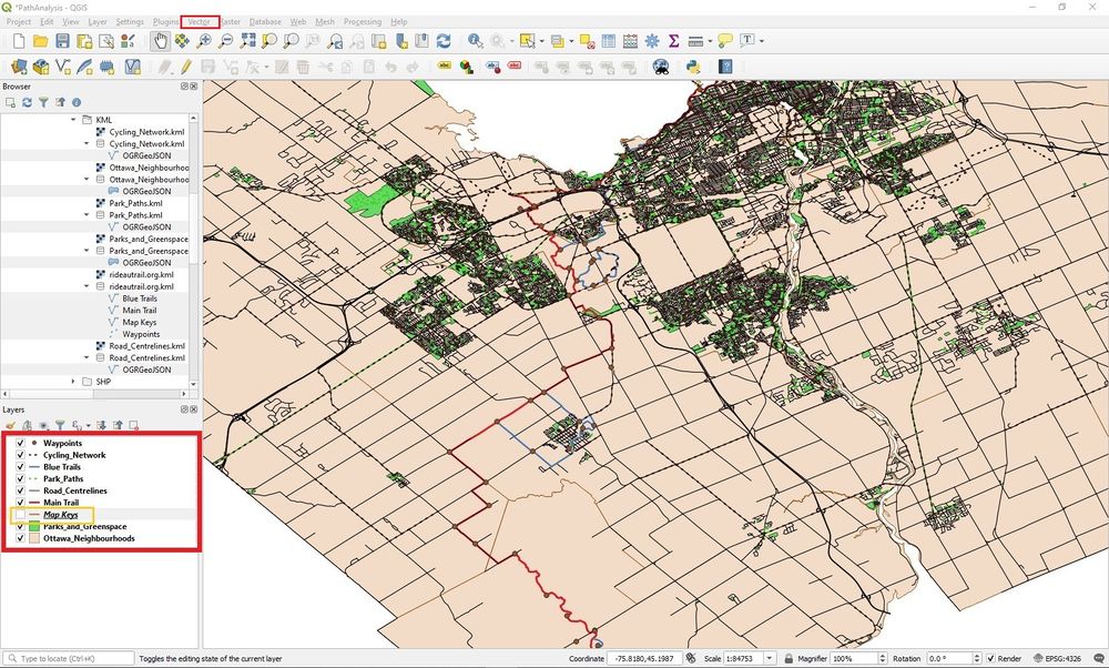
We will now conduct the path analysis of intersections to the main trail. Click the tab Vector > Analysis Tools > Line intersections...
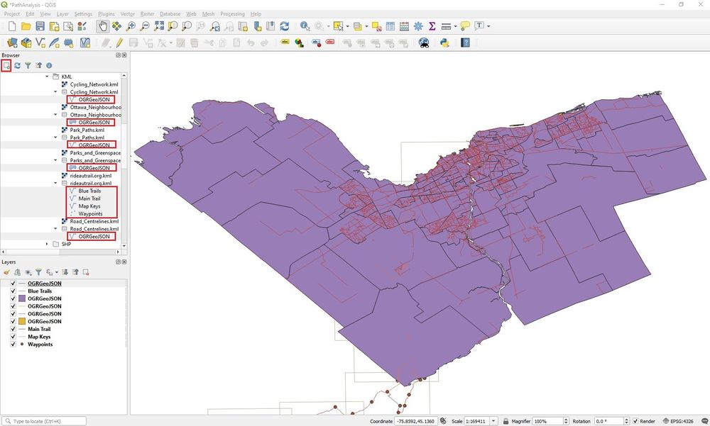
Figure 3. Add the OGRGeoJson files to the map. GeoJSON supports a variety of geometry types, which includes Point, LineString, Polygon, MultiPoint, MultiLineString, and MultiPolygon. It is a format for encoding geographic data.
Figure 4. Once the data is added, it is recommended that you make changes to the layers, so it can be viewed more easily.
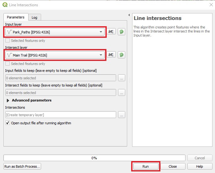
A window will open. Select the input layer accordingly. The intersect layer will be the main trail. This process will be repeated with the other line layers for the input layer. Click run.
Figure 5. Once you select run, the output will be displayed in the layers section, given that the input layer and intersect layer is selected accordingly.
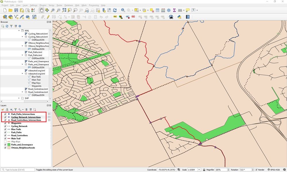
Once the multiple analyses are completed, change the symbols for easier viewing. you will now be able to see where various lines intersect with the main trail. The line intersections tool can be used to identify any paired combination of lines.
Figure 6. Results from using the line intersections tool.
All the information that results from the analysis can be viewed in an attribute table. This information is in the new layer that was created. In this case it is the intersections layers. The attribute table will provide valuable geographic information such as how to access the points, road type and length of the line that the point is found on. To open the attribute table, right click the layer and select open attribute table.
Figure 7. An opened attribute table for the layer Road_Centrelines_Intersections. In this attribute table, geographic information such as road name in which the intersection point is located on, name of accessing roads and length of road. This information can be useful when planning a trip.
Cross-Referencing With Other Maps
Please turn on the map keys layer and open the link Rideau Trail in the reference section. We will now cross-reference our information with maps provided by the Rideau Trail Association. Link to the maps are found in the reference section.
Figure 8. Map keys will be used for further viewing of the area.
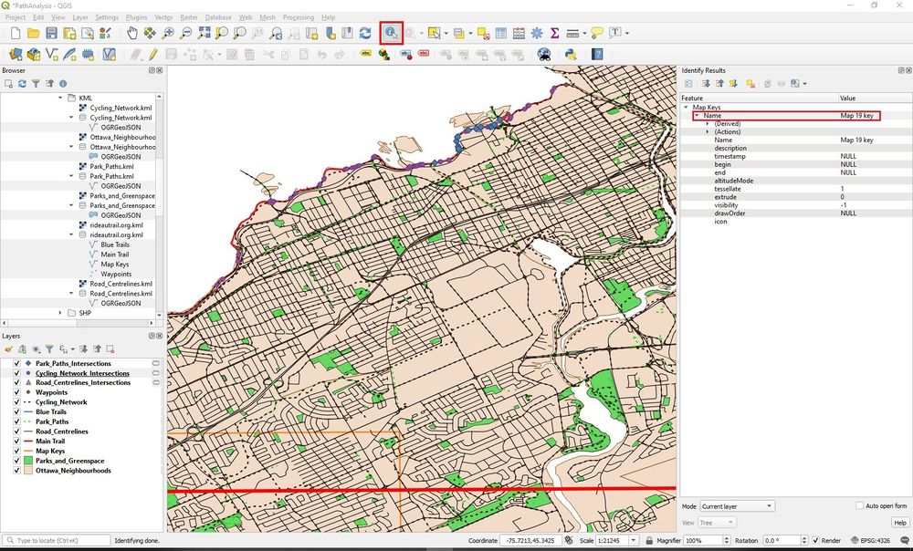
Select Identify Features. Go to an area of interest in which intersections have been identified. Select the map key on the map, it will identify the map key that will be required from the Rideau Trail Association website.
Figure 9. Identify the map key required the area of interest.
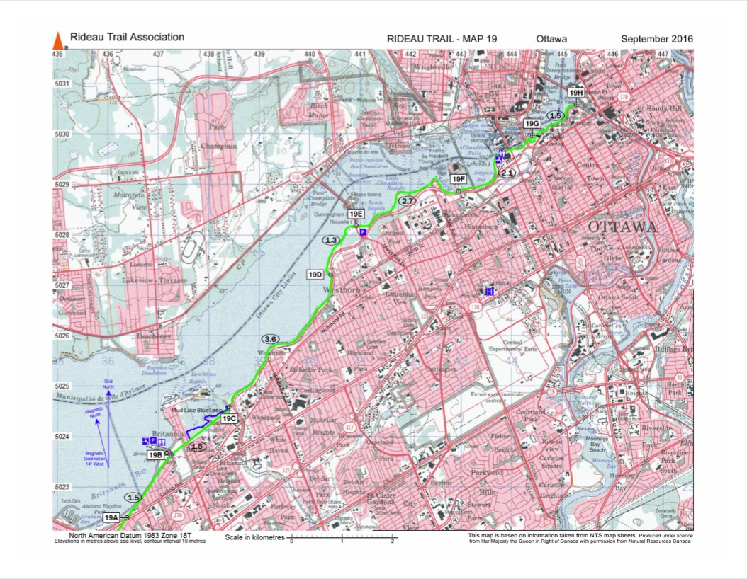
Select the required map from the Rideau Trail Association website from the link in the reference section.
Figure 10. View the area in another type of map. It may provide more useful information for the area.
View in Google Earth Pro
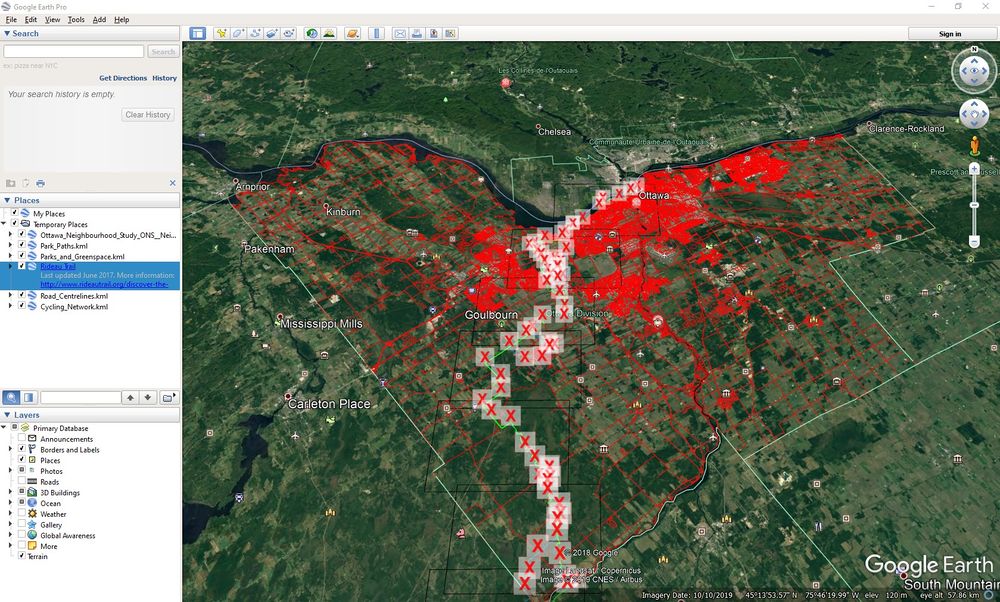
Since the data is KML, it can be viewed in Google Earth Pro.
Figure 11. The same data that was used in the previous analysis can be read in Google Earth Pro.
Shortest Path Analysis
Using the intersections layers created in the Process section, we will now use a Network Analysis tool within QGIS to calculate the shortest path between any random point in Ottawa and the intersection points of The Rideau Trail. Say you wanted to access The Rideau Trail from Carleton Universtiy, but you only wanted to travel along the roads to get to it. In this scenario, we will be using the Roads_Centrelines layer and the Roads_Centreline_Intersections points that were previously created to find the shortest distances possible to each of the places where a road and The Rideau Trail intersect. This analysis aims to answer the question, how do I get to the Rideau Trail using roads from my location in Ottawa?
NOTE: This analysis was conducted using QGIS 3.4.
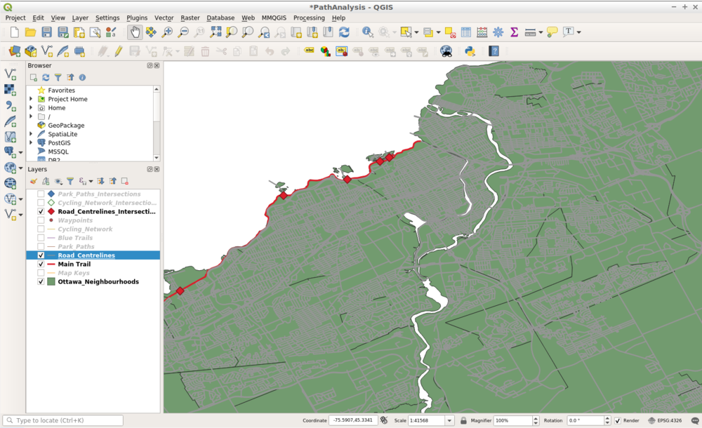
Figure 12. Start by having your Road_Centrelines_Intersections, Road_Centrelines, Main Trail, and Ottawa_Neighbourhoods layers turned on with easy to view symbology.
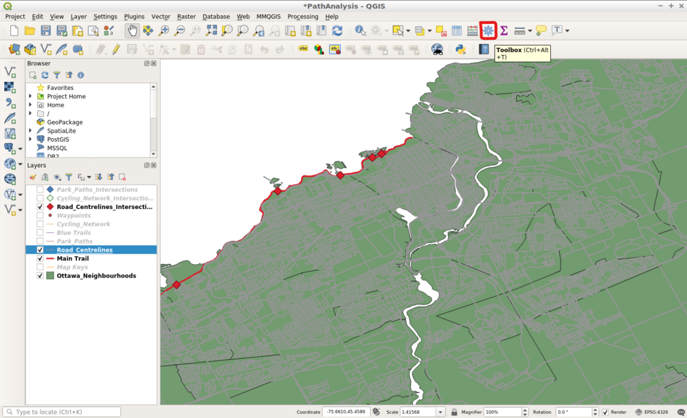
Next, open the QGIS toolbox by clicking the gear icon on the Attributes toolbar. If you cannot find this icon, go to Processing > Toolbox.
Figure 13. The location of the Toolbox icon on the Attributes toolbar.
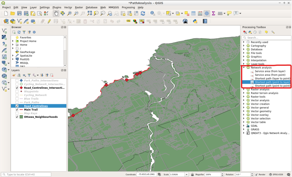
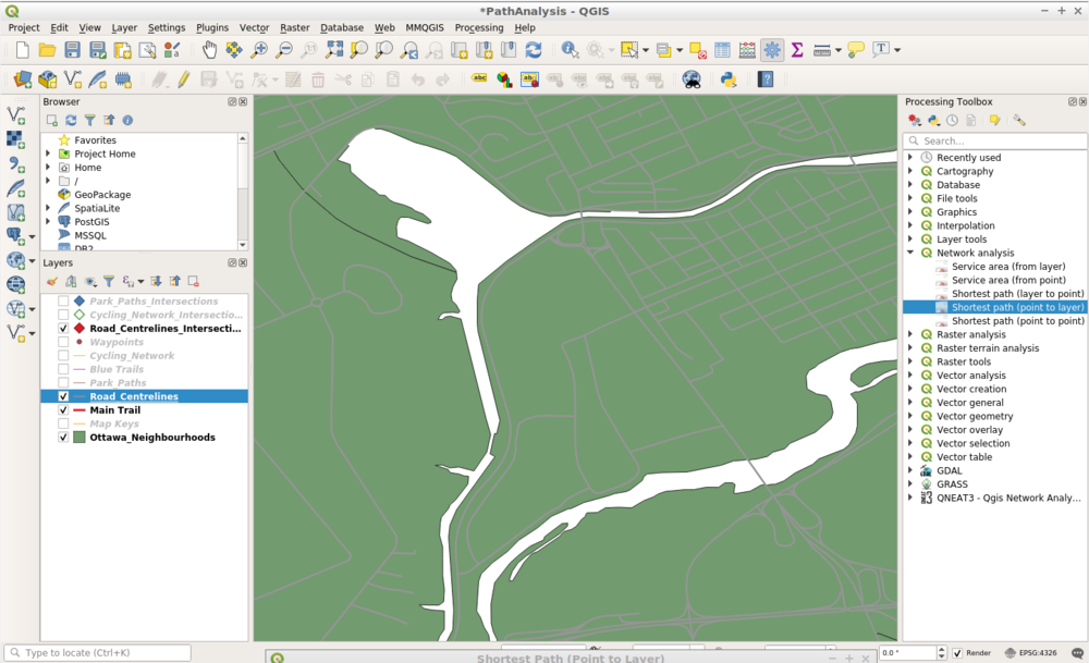
After clicking the Toolbox, click on the drop-down menu beside Network analysis. There will be several options, but click on the Shortest path (point to layer) tool. The Shortest path (point to layer) tool is an algorithm that calculates the shortest path between a given start point and multiple end points using a vector layer.
Figure 14. The location of the Shortest path (point to layer) tool in the Network analysis toolbox.
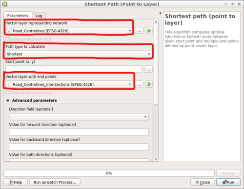
Clicking on the Shortest path (point to layer) tool will bring up a separate window. In the Parameters window, the Vector layer representing network will be the Road_Centrelines layer. The Path type to calculate will be Shortest. The Vector layer with end points will be the Roads_Centerlines_Intersections layer.
Figure 15. The desired configuration in the parameters window.
Before hitting Run, you will have to select a starting point for the algorithm to calculate the shortest distance. In the parameters window, click on the Start point (x, y). This will minimize the window to your map view, and your cursor will be a cross hair. Select an area on Carleton University's campus.
Figure 16. Selecting a desired start point on Carleton University's campus.
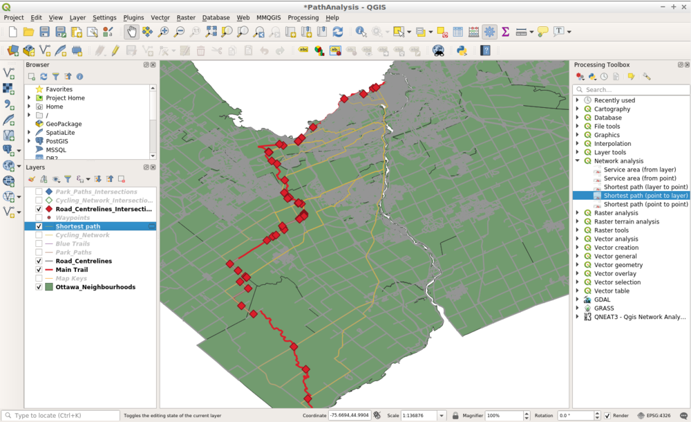
Once you have selected a starting point, the Shortest path (point to layer) window will maximize, and you may now hit the Run function in the bottom right corner of the window. Running this tool will create a temporary layer, and will demonstrate all the different shortest pathway possibilities to get to any of the locations where the road intersects The Rideau Trail as if you were travelling by the Roads_Centrelines layer.
Figure 17. A screenshot of the layer created by the Shortest path (point to layer) tool. This layer displays all of the shortest pathways from the chosen start point at Carleton University to each location where the Road_Centrelines layer intersects the Main Trail (Rideau Trail).
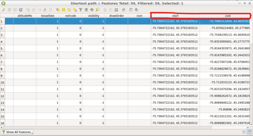
Opening up the attribute table of the new Shortest path layer will reveal several attribute columns, however, the columns of most interest include the start and cost columns. The start and cost columns represent the distance between the start point (start) and the end point (cost) in layer units. In this case, the start and the cost are represented in latitude and longitude coordinates. If interested, you can use these coordinates to calculate the exact distance between each start and end point.
Figure 18. The start and cost columns in the attribute table of the Shortest path layer.
This analysis can be completed using any of the other path network and intersection layers as well.
References
ESRI. (1998). ESRI Shapefile Technical Description (PDF). Retrieved from https://www.esri.com/library/whitepapers/pdfs/shapefile.pdf
Google Developers. (2019). Keyhole Markup Language. Retrieved from https://developers.google.com/kml
GeoJson. (2019). GeoJson. Retrieved from https://geojson.org/
Rideau Trail Association. (2019). Discover the Trail. Retrieved from https://www.rideautrail.org/discover-the-trail/maps/


