Difference between revisions of "Calculating Street Intersection Density in QGIS"
| (15 intermediate revisions by the same user not shown) | |||
| Line 1: | Line 1: | ||
==Introduction== |
==Introduction== |
||
===Purpose=== |
===Purpose=== |
||
Street intersection density is a useful measure of network connectivity. This tutorial will show how to calculate street intersection density using QGIS. The analysis of calculating street intersection density is commonly used in transportation design, to scope out the best walkability of neighbourhoods and bike paths. This tutorial aims to demonstrate how to use spatial analysis in understanding spatial patterns for urban accessibility while also learning how to use an open-source GIS software |
Street intersection density is a useful measure of network connectivity. This tutorial will show how to calculate street intersection density using QGIS. The analysis of calculating street intersection density is commonly used in transportation design, to scope out the best walkability of neighbourhoods and bike paths. This tutorial aims to demonstrate how to use spatial analysis in understanding spatial patterns for urban accessibility while also learning how to use an open-source GIS software. In the end, creating a map showing intersection density across a city. This is useful especially for people in urban planning and land use planning but each task could be used in other aspects (such as individual projects, educational purposes etc.) as well. |
||
For example, this tutorial will be calculating the street intersection density of the city of Ottawa. |
For example, this tutorial will be calculating the street intersection density of the city of Ottawa. |
||
===About QGIS=== |
===About QGIS=== |
||
QGIS (Quantum GIS) is a free and open-source GIS program released under the GNU General Public License. It has a wide variety of features |
QGIS (Quantum GIS) is a free and open-source GIS program released under the GNU General Public License. It has a wide variety of features from creating, editing, visualizing, analyzing and publishing of spatial data <ref>QGIS: Defining what is QGIS https://www.qgis.org/en/site/about/index.html</ref>. In the context of this tutorial, vector data editing and creating grids will be demonstrated. QGIS is available for download on a variety of operating systems from Windows, Mac, Linux, BSD and mobile devices. |
||
===''Note''=== |
===''Note''=== |
||
The QGIS version used here in this tutorial is 3. |
The QGIS version used here in this tutorial is 3.16 (the latest version as of December 2021) on a Windows operating system. When trying this tutorial, if you are using a previous or updated version of QGIS or on a different operating system, please keep in mind there may be differences in the figures and instructions shown in this tutorial. |
||
==Getting Started== |
==Getting Started== |
||
| Line 16: | Line 16: | ||
===Finding Data=== |
===Finding Data=== |
||
Data for this tutorial was found through the City of Ottawa's Open Data Website <ref>Open Ottawa: Data retrieval https://open.ottawa.ca/</ref>. [https://open.ottawa.ca/ HERE] |
|||
However, to acquire spatial data for use in QGIS for other cities, there are many open data resources including Open Data Catalogues, Open City, GeoHub etc. A simple Google search with the name of the city and the words “open data” next to it should give you at least a couple options. |
|||
Follow along into the next section to learn how to do this tutorial step by step. |
|||
==Tutorial== |
==Tutorial== |
||
===Download Data=== |
===Download Data=== |
||
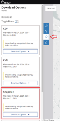
[[File:OttawaWards.png|200px|thumb|right|Figure 1. Downloading Wards file from Open Ottawa.]] |
|||
===Clipping The Road Network to the City Boundary=== |
|||
The two datasets we will need are: |
|||
: 1. The city boundary of Ottawa which can be found by searching '''Wards''' or click on this direct link [https://open.ottawa.ca/datasets/wards/explore?location=45.249481%2C-75.800844%2C1.72 HERE]. Download in Shapefile format (see Figure 1). |
|||
: 2. The road centerlines within the City of Ottawa can be found searching '''Centrelines''' or click on this direct link [https://open.ottawa.ca/datasets/road-centrelines/explore?location=45.245850%2C-75.794650%2C1.68 HERE]. Download in Shapefile format (same as downloading Wards file, see Figure 1 for reference). |
|||
Extract (unzip) both folders and save in the working directory you will be using. |
|||
===Extracting Road Intersections=== |
|||
The first step is to extract the road intersections. |
|||
: 1. To begin, import both shapefiles into QGIS. Go to the '''Browser Panel''' (on the left of your new project screen) then navigate to where you stored the 2 shapefiles from your working directory. Drag and drop both shapefiles to the '''Layers''' panel. |
|||
With these files, because of the algorithm, there are some intersections considered as a valid intersection but are only a single line segment. For analyzing street intersection density, we need to extract only the intersections when 2 or more streets intersect. To do this, we need to merge all adjacent road segments. |
|||
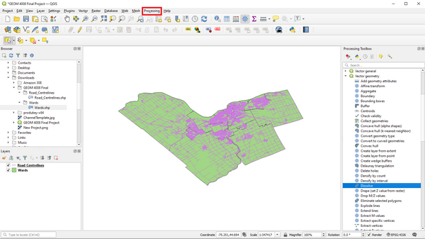
: 2. Open the '''Processing > Toolbox''' (along the top row) and locate '''Vector geometry''' then double click on '''Dissolve''' (see Figure 2). |
|||
[[File:ERI2.png|600px|thumb|center|Figure 2. Finding Processing Toolbox and Dissolve tool.]] |
|||
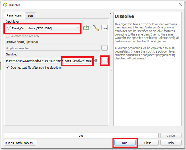
: 3. In the Input layer, select '''''Roads_Centrelines'''''. In the Dissolved output layer, click on the three dots (shown in Figure 3) and then '''Save to File...''' enter '''''Roads_Dissolved'''''. Hit '''Run''' to process. |
|||
[[File:ERI3.png|600px|thumb|center|Figure 3. Inputs for Dissolve tool]] |
|||
Now, you will have a layer with all the road segments merged into a single feature. Next, we will be creating a layer that has all adjacent segments merged. |
|||
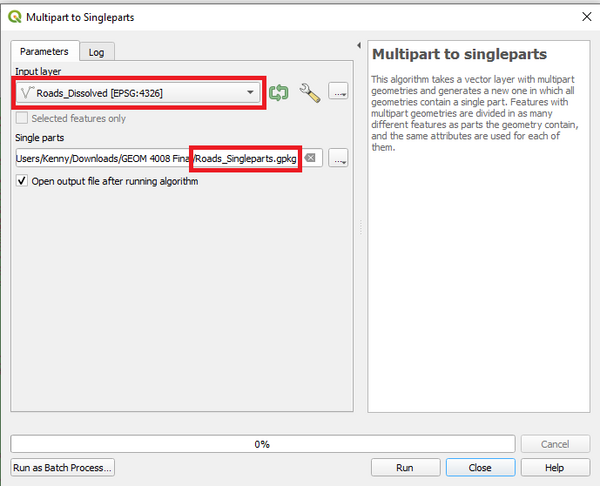
: 4. Similar to the previous step, go back into '''Vector geometry''' locate '''Multipart to singleparts''' and double-click. Select the layer '''''Roads_Dissolved''''' as the Input layer. Enter '''''Roads_Singleparts''''' as the Single parts output. Click '''Run''' (see Figure 4 for reference). |
|||
[[File:Multipartstos.png|600px|thumb|center|Figure 4. Inputs for Multipart to Singleparts tool.]] |
|||
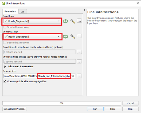
: 5. Now, open the '''Processing Toolbox''' and locate '''Vector overlay''' double-click on '''Line intersections'''. Select '''''Roads_Singleparts''''' as both the Input and Intersect layer. Name the Intersections output layer as '''''Roads_Line_Intersections'''''. Hit '''Run''' (see Figure 5 for reference). This may take a couple minutes as it is a computationally intensive operation. |
|||
[[File:ERI5.png|600px|thumb|center|Figure 5. Inputs for Line intersections tool. ]] |
|||
All the intersections are now correctly identified. However, there are a Few duplicate points from adjacent segments. We will need to remove these duplicates as we do not want an inflated number of intersections. |
|||
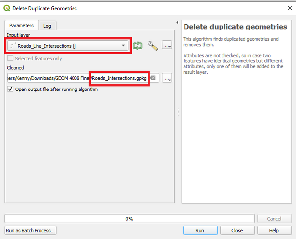
: 6. Still in the '''Processing Toolbox''' locate '''Vector general''' and double-click on '''Delete duplicate geometries'''. Select '''''Roads_Line_Intersections''''' as the Input layer and enter '''''Roads_Intersections''''' as the Cleaned output layer. Hit the '''Run''' button (see Figure 6 for reference). |
|||
[[File:ERI6.png|600px|thumb|center|Figure 6. Inputs for Delete duplicate geometries tool.]] |
|||
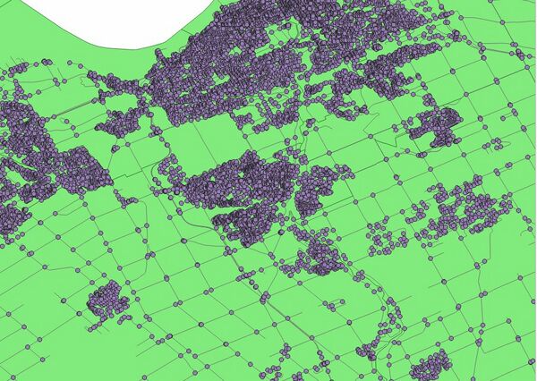
: 7. It is possible to remove the layers we do not need anymore, which are the layers '''''Roads_Line_Intersections''''', '''''Roads_Dissolved''''' and '''''Roads_Centrelines'''''. Simply right-click on each and select '''Remove layer'''. So far, the map should look like Figure 7. |
|||
[[File:Map.jpg|600px|thumb|center|Figure 7. Map with layers '''''Roads_Line_Intersections''''', '''''Roads_Singleparts''''' and '''''Wards'''''. ]] |
|||
===Creating a Grid=== |
|||
To display the density of points, one of the best visually appealing ways to do so is creating a grid. We will do this by overlaying a regular grid and counting points in each grid polygon. |
|||
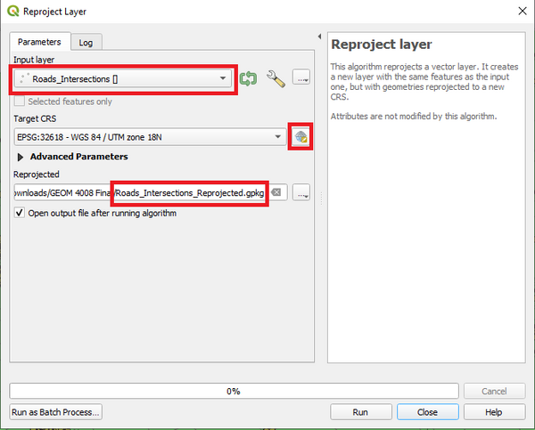
: 1. First, we need to reproject the data to a projected CRS (coordinate reference system) to be able to use linear units of measurements. Open the '''Processing Toolbox''' locate '''Vector general''' click '''Reproject layer'''. If you are looking to figure out where your city is located on the UTM zone, click on this link [https://mangomap.com/robertyoung/maps/69585/what-utm-zone-am-i-in-# HERE]<ref>Mango: Finding UTM zone of a city https://mangomap.com/robertyoung/maps/69585/what-utm-zone-am-i-in-#</ref>. In my case, Ottawa is located in the UTM Zone 18N. Select '''''Roads_Intersections''''' as the Input layer. Under Target CRS, search using the globe icon (see Figure 8) and select '''WGS 84 / UTM zone 18N'''. Enter the Reprojected output layer as '''''Roads_Intersections_Reprojected''''' then click '''Run'''. |
|||
[[File:Reprojection.png|600px|thumb|center|Figure 8. Inputs for Reproject layer tool. ]] |
|||
: 2. Now that the '''''Roads_Intersections_Reprojected''''' layer is added, right-click and select '''Layer CRS''' then to '''Set Project CRS from Layer'''. and remove the '''''Roads_Intersections''''' layer. |
|||
With the map now reprojected, it is time to create the grid. |
|||
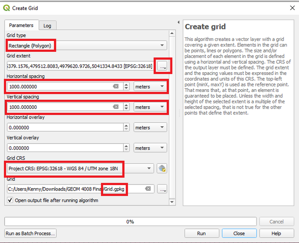
: 3. Open the '''Processing Toolbox''' find '''Vector creation''' and double-click '''Create grid'''. Select Grid type as '''Rectangle (Polygon)'''. Using the '''...''' button in Grid extent (see in Figure 9), select '''Calculate from Layer''' then click on '''''Roads_Intersections_Reprojected'''''. We are creating a grid of of 1km x 1km, so set both Horizontal spacing and Vertical spacing as 1000 meters. In the Grid CRS select '''Project CRS'''. Save the Grid output layer as '''''Grid''''' . Last but not least, click '''Run'''. |
|||
[[File:Grid.png|600px|thumb|center|Figure 9. Inputs for Create grid tool. ]] |
|||
The '''''Grid''''' layer containing rectangular grid polygons is now created. Next we will count the number of points in each polygon. |
|||
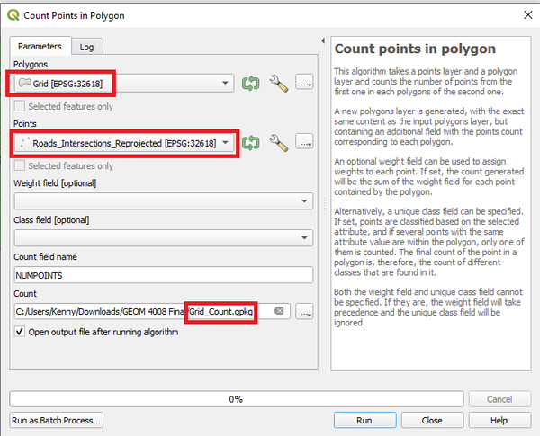
: 4. Open the '''Processing Toolbox''', locate '''Vector analysis''' and click on '''Count points in polygon'''. Select '''''Grid''''' as the Polygons layer and '''''Roads_Intersections_Reprojected''''' as the Points layer. Save the Count output layer as '''''Grid_Count'''''. Click '''Run''' (see Figure 10 for reference). |
|||
[[File:GridCount.png|600px|thumb|center|Figure 10. Inputs for Count points in polygon tool. ]] |
|||
The layer '''''Grid_Count''''' now has the attribute NUMPOINTS which contains the number of intersection points in each grid. There are many grids with 0 points so let's remove the grid polygons that contain no intersections as that is not needed for this analysis. |
|||
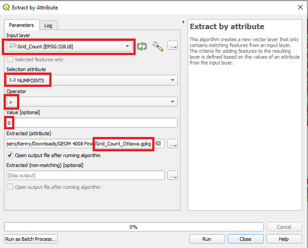
: 5. Open the '''Processing Toolbox''', locate '''Vector selection''' and double-click on '''Extract by attribute'''. Select '''''Grid_Count''''' as the Input layer, then select '''NUMPOINTS''' in Selection attribute, '''>''' in Operator and enter the Value as '''0'''. Save the Extracted (attribute) output layer as '''''Grid_Count_Ottawa''''' Click '''Run''' (see Figure 11). |
|||
[[File:GridCountOtt.png|600px|thumb|center|Figure 11. Inputs for Extract by attribute tool. ]] |
|||
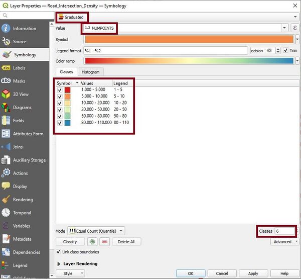
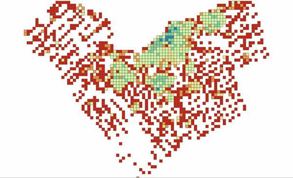
: 6. Final steps are to remove all layers except for '''''Grid_Count_Ottawa''''' and rename it to '''''Road_Intersection_Density'''''. Changing up the symbology to make the density of each grid stand out is very important. To do this, double-click on the '''''Road_Intersection_Density''''' layer. The Layer Properties screen should pop up and from here go to '''Symbology''' and change everything to your liking. For my map, I chose to do a graduated renderer with 6 classes. (see Figure 12 for all of the changes I made to my map and Figure 13 for my final product). |
|||
[[File:Symbologyy.jpg|600px|thumb|center|Figure 12. The symbology used to create the final product. ]] |
|||
[[File:FinishedMap.jpg|600px|thumb|center|Figure 13. The final map showing intersection density across the city of Ottawa. ]] |
|||
Congrats! You have made it to the end of this tutorial, you have now created a map showing intersection density across the city of Ottawa or the city of your choice. |
|||
==Conclusion== |
|||
==Resources== |
==Resources== |
||
Latest revision as of 09:36, 25 December 2021
Contents
Introduction
Purpose
Street intersection density is a useful measure of network connectivity. This tutorial will show how to calculate street intersection density using QGIS. The analysis of calculating street intersection density is commonly used in transportation design, to scope out the best walkability of neighbourhoods and bike paths. This tutorial aims to demonstrate how to use spatial analysis in understanding spatial patterns for urban accessibility while also learning how to use an open-source GIS software. In the end, creating a map showing intersection density across a city. This is useful especially for people in urban planning and land use planning but each task could be used in other aspects (such as individual projects, educational purposes etc.) as well.
For example, this tutorial will be calculating the street intersection density of the city of Ottawa.
About QGIS
QGIS (Quantum GIS) is a free and open-source GIS program released under the GNU General Public License. It has a wide variety of features from creating, editing, visualizing, analyzing and publishing of spatial data [1]. In the context of this tutorial, vector data editing and creating grids will be demonstrated. QGIS is available for download on a variety of operating systems from Windows, Mac, Linux, BSD and mobile devices.
Note
The QGIS version used here in this tutorial is 3.16 (the latest version as of December 2021) on a Windows operating system. When trying this tutorial, if you are using a previous or updated version of QGIS or on a different operating system, please keep in mind there may be differences in the figures and instructions shown in this tutorial.
Getting Started
Acquiring QGIS
To begin, download the latest version of QGIS on your operating system. QGIS is available for download on their website. HERE
Finding Data
Data for this tutorial was found through the City of Ottawa's Open Data Website [2]. HERE
However, to acquire spatial data for use in QGIS for other cities, there are many open data resources including Open Data Catalogues, Open City, GeoHub etc. A simple Google search with the name of the city and the words “open data” next to it should give you at least a couple options.
Follow along into the next section to learn how to do this tutorial step by step.
Tutorial
Download Data
The two datasets we will need are:
- 1. The city boundary of Ottawa which can be found by searching Wards or click on this direct link HERE. Download in Shapefile format (see Figure 1).
- 2. The road centerlines within the City of Ottawa can be found searching Centrelines or click on this direct link HERE. Download in Shapefile format (same as downloading Wards file, see Figure 1 for reference).
Extract (unzip) both folders and save in the working directory you will be using.
Extracting Road Intersections
The first step is to extract the road intersections.
- 1. To begin, import both shapefiles into QGIS. Go to the Browser Panel (on the left of your new project screen) then navigate to where you stored the 2 shapefiles from your working directory. Drag and drop both shapefiles to the Layers panel.
With these files, because of the algorithm, there are some intersections considered as a valid intersection but are only a single line segment. For analyzing street intersection density, we need to extract only the intersections when 2 or more streets intersect. To do this, we need to merge all adjacent road segments.
- 2. Open the Processing > Toolbox (along the top row) and locate Vector geometry then double click on Dissolve (see Figure 2).
- 3. In the Input layer, select Roads_Centrelines. In the Dissolved output layer, click on the three dots (shown in Figure 3) and then Save to File... enter Roads_Dissolved. Hit Run to process.
Now, you will have a layer with all the road segments merged into a single feature. Next, we will be creating a layer that has all adjacent segments merged.
- 4. Similar to the previous step, go back into Vector geometry locate Multipart to singleparts and double-click. Select the layer Roads_Dissolved as the Input layer. Enter Roads_Singleparts as the Single parts output. Click Run (see Figure 4 for reference).
- 5. Now, open the Processing Toolbox and locate Vector overlay double-click on Line intersections. Select Roads_Singleparts as both the Input and Intersect layer. Name the Intersections output layer as Roads_Line_Intersections. Hit Run (see Figure 5 for reference). This may take a couple minutes as it is a computationally intensive operation.
All the intersections are now correctly identified. However, there are a Few duplicate points from adjacent segments. We will need to remove these duplicates as we do not want an inflated number of intersections.
- 6. Still in the Processing Toolbox locate Vector general and double-click on Delete duplicate geometries. Select Roads_Line_Intersections as the Input layer and enter Roads_Intersections as the Cleaned output layer. Hit the Run button (see Figure 6 for reference).
- 7. It is possible to remove the layers we do not need anymore, which are the layers Roads_Line_Intersections, Roads_Dissolved and Roads_Centrelines. Simply right-click on each and select Remove layer. So far, the map should look like Figure 7.
Creating a Grid
To display the density of points, one of the best visually appealing ways to do so is creating a grid. We will do this by overlaying a regular grid and counting points in each grid polygon.
- 1. First, we need to reproject the data to a projected CRS (coordinate reference system) to be able to use linear units of measurements. Open the Processing Toolbox locate Vector general click Reproject layer. If you are looking to figure out where your city is located on the UTM zone, click on this link HERE[3]. In my case, Ottawa is located in the UTM Zone 18N. Select Roads_Intersections as the Input layer. Under Target CRS, search using the globe icon (see Figure 8) and select WGS 84 / UTM zone 18N. Enter the Reprojected output layer as Roads_Intersections_Reprojected then click Run.
- 2. Now that the Roads_Intersections_Reprojected layer is added, right-click and select Layer CRS then to Set Project CRS from Layer. and remove the Roads_Intersections layer.
With the map now reprojected, it is time to create the grid.
- 3. Open the Processing Toolbox find Vector creation and double-click Create grid. Select Grid type as Rectangle (Polygon). Using the ... button in Grid extent (see in Figure 9), select Calculate from Layer then click on Roads_Intersections_Reprojected. We are creating a grid of of 1km x 1km, so set both Horizontal spacing and Vertical spacing as 1000 meters. In the Grid CRS select Project CRS. Save the Grid output layer as Grid . Last but not least, click Run.
The Grid layer containing rectangular grid polygons is now created. Next we will count the number of points in each polygon.
- 4. Open the Processing Toolbox, locate Vector analysis and click on Count points in polygon. Select Grid as the Polygons layer and Roads_Intersections_Reprojected as the Points layer. Save the Count output layer as Grid_Count. Click Run (see Figure 10 for reference).
The layer Grid_Count now has the attribute NUMPOINTS which contains the number of intersection points in each grid. There are many grids with 0 points so let's remove the grid polygons that contain no intersections as that is not needed for this analysis.
- 5. Open the Processing Toolbox, locate Vector selection and double-click on Extract by attribute. Select Grid_Count as the Input layer, then select NUMPOINTS in Selection attribute, > in Operator and enter the Value as 0. Save the Extracted (attribute) output layer as Grid_Count_Ottawa Click Run (see Figure 11).
- 6. Final steps are to remove all layers except for Grid_Count_Ottawa and rename it to Road_Intersection_Density. Changing up the symbology to make the density of each grid stand out is very important. To do this, double-click on the Road_Intersection_Density layer. The Layer Properties screen should pop up and from here go to Symbology and change everything to your liking. For my map, I chose to do a graduated renderer with 6 classes. (see Figure 12 for all of the changes I made to my map and Figure 13 for my final product).
Congrats! You have made it to the end of this tutorial, you have now created a map showing intersection density across the city of Ottawa or the city of your choice.
Resources
- ↑ QGIS: Defining what is QGIS https://www.qgis.org/en/site/about/index.html
- ↑ Open Ottawa: Data retrieval https://open.ottawa.ca/
- ↑ Mango: Finding UTM zone of a city https://mangomap.com/robertyoung/maps/69585/what-utm-zone-am-i-in-#
