Difference between revisions of "Kriging Interpolation Comparison on Alberta Weather Station Elevation Data using System for Automated Geoscientific Analysis (SAGA GIS)"
Alex Fortin (talk | contribs) m |
Pulsiferpl (talk | contribs) m (→Conclusion) |
||
| (62 intermediate revisions by 3 users not shown) | |||
| Line 1: | Line 1: | ||
<big>Kriging Interpolation Comparison on Alberta Weather Station Elevation Data using System for Automated Geoscientific Analysis (SAGA GIS)</big> |
<big>Kriging Interpolation Comparison on Alberta Weather Station Elevation Data using System for Automated Geoscientific Analysis (SAGA GIS)</big> |
||
='''Introduction'''= |
|||
==Purpose== |
==Purpose== |
||
The purpose of this tutorial is to provide a step-by-step guide to using the Kriging interpolation technique in SAGA GIS, a software that many users may not have encountered before. The tutorial will introduce the various types of Kriging and the key variables to consider during the process. By comparing results from a dataset with dense data points to one with sparse data, the tutorial aims to highlight the critical role that data quality and quantity play in achieving accurate interpolation results. |
The purpose of this tutorial is to provide a step-by-step guide to using the Kriging interpolation technique in SAGA GIS, a software that many users may not have encountered before. The tutorial will introduce the various types of Kriging and the key variables to consider during the process. By comparing results from a dataset with dense data points to one with sparse data, the tutorial aims to highlight the critical role that data quality and quantity play in achieving accurate interpolation results. |
||
| Line 15: | Line 15: | ||
* Run the saga_gui.exe to open the program |
* Run the saga_gui.exe to open the program |
||
='''Data'''= |
|||
'''Transformed Data used in tutorial is available in the '''''Download Tutorial Data''''' section''' |
|||
==Acquiring the Data== |
==Acquiring the Data== |
||
To download the <b> |
To download the <b>Elevation</b> data follow these steps: |
||
* Visit the [https://geo1.scholarsportal.info/#_lang=en <b>Scholars GeoPortal</b>]. |
|||
* Visit the <b>Significant Earthquake Database</b> at this link [https://www.ngdc.noaa.gov/hazel/view/hazards/earthquake/search] |
|||
* In the search bar enter <b> Weather Stations </b>. |
|||
* Fill in the date of the form beginning by setting the minimum year to <b>1990</b> and the maximum year to <b>2013</b> |
|||
* The Canadian Weather Stations should be available to <b> Add </b> to map. |
|||
* Select <b>North America and Hawaii</b> as the Region Name |
|||
* After adding the data to the map it is possible to select an area. In our case we selected All of Alberta's data. |
|||
* Once this is completed, go to the <b> Download </b> page and either download your selected area or the entire dataset. |
|||
<br> |
|||
To download the <b>Alberta</b> boundary file follow these steps: |
|||
* Visit the [https://open.canada.ca/data/en/dataset/a883eb14-0c0e-45c4-b8c4-b54c4a819edb/resource/12c03de6-c3f7-4f5f-bb5c-d479f2332842 <b>Open Canada</b>] |
|||
* Download the '''Provinces/Territories, Cartographic Boundary File - 2016 Census''' |
|||
* Clip to only Alberta or Province of choice. ''(Clipped Data Available In Download Tutorial Data Section)'' |
|||
<br> |
|||
To download the <b>Alberta 25M Digital Elevation Model</b> follow these steps: |
|||
* Go to [https://www.altalis.com/map;id=150 Altalis.com] |
|||
*Create ''Altalis'' account to download the free 25M Digital Elevation Model |
|||
*Add the 25M Raster DEM to your cart. |
|||
* Go to cart and Proceed with Download. |
|||
* An email with your file ready to download will be sent to you shortly. |
|||
==Download Tutorial Data== |
|||
All the data and code can be downloaded from this [https://drive.google.com/drive/folders/10vHdF1R7j88iQ2xJ6KoINM0LUkJsvLiq?usp=sharing Google Drive Link] <br> |
|||
The download contains: <br> |
|||
TutorialDataDownload.zip (124KB) |
|||
* Alberta Boundary Shapefile (152KB) <ref>https://open.canada.ca/data/en/dataset/a883eb14-0c0e-45c4-b8c4-b54c4a819edb/resource/12c03de6-c3f7-4f5f-bb5c-d479f2332842</ref> |
|||
* Alberta Weather Station Data (100KB) <ref>https://geo1.scholarsportal.info/#_lang=en</ref> |
|||
* Limited Alberta Weather Station Data (30.4KB) <ref>https://geo1.scholarsportal.info/#_lang=en</ref> |
|||
AlbertaDEM.zip(1.18GB) *Optional |
|||
* Alberta 25M Digital Elevation Model (8.25GB) <ref>https://www.altalis.com/map;id=150</ref> |
|||
='''Tutorial'''= |
|||
==SAGA GIS Interpolation Options== |
|||
Saga has four different types of interpolation, each with their own strengths, weaknesses and specific characterstics. We will explain the use cases of each of them. They also have a 3D Kriging tool that we will not go into detail in this tutorial. There are also lots of different options and inputs that modify the kriging in SAGA which we will explain and how they impact the interpolation. |
|||
*''' Ordinary Kriging''' |
|||
** Assumptions: Assumes the mean of the data is unknown but constant over the area of interest. |
|||
** Advantages: Simple, widely applicable, and does not require external data or a predefined trend. |
|||
** Use Case: Best for spatially autocorrelated data with no obvious trends or external influencing factors. |
|||
*''' Regression Kriging''' |
|||
** Assumptions: Combines a deterministic regression model with kriging of residuals. |
|||
** Advantages: Incorporates additional explanatory variables (e.g., slope, aspect) to improve accuracy. |
|||
** Use Case: Ideal when auxiliary data strongly influences the spatial distribution of the variable. |
|||
*''' Simple Kriging''' |
|||
** Assumptions: Assumes a known and constant mean across the study area. |
|||
** Advantages: Computationally efficient and straightforward but requires prior knowledge of the mean. |
|||
** Use Case: Rarely used unless the mean is well-established (e.g., synthetic datasets). |
|||
*'''Universal Kriging''' |
|||
** Assumptions: Assumes the data has a deterministic trend (e.g., polynomial or linear) over space. |
|||
** Advantages: Models and accounts for spatial trends while still relying on kriging for local variation. |
|||
** Use Case: Useful for non-stationary data with a noticeable trend (e.g., elevation gradients across a region). |
|||
==Kriging Interpolation Step-By-Step== |
|||
'''Step 1: Open the Data Files''' |
|||
* Navigate to '''''File''''' → '''''Open'''''. |
|||
* Open each data file individually. (the files with .shp file format) |
|||
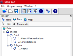
* Ensure all the data has been added correctly. Go to the Manager tab → Data → Tree |
|||
::[[Image:SAGApic1.png|thumb|none|frame|''Figure 1: Data Successfully Imported'']] |
|||
<br> |
|||
'''Step 2: Add Files to the Map''' |
|||
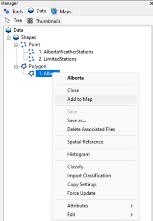
* Right-click on each file and select '''''Add to Map'''''. |
|||
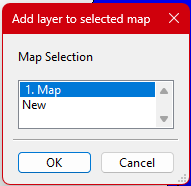
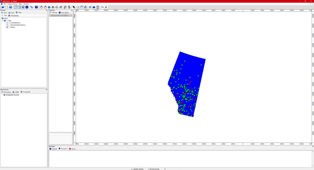
* Ensure that all files are added to the same map. Avoid creating separate maps for each file. ('' See ''Figure 2 through 4'' for the exact steps and expected outcome.'') |
|||
::[[Image:SAGApic2.png|thumb|none|frame|''Figure 2: Adding Files to a Map'']] |
|||
::[[Image:SAGApic3.png|thumb|none|frame|''Figure 3: Choose the Desired Map'']] |
|||
::[[Image:SAGApic4.png|thumb|none|frame|1000px|''Figure 4: Expected Outcome'']] |
|||
<br> |
|||
'''Step 3: Kriging Analysis Setup''' |
|||
* Go to '''''Geoprocessing''''' tab. |
|||
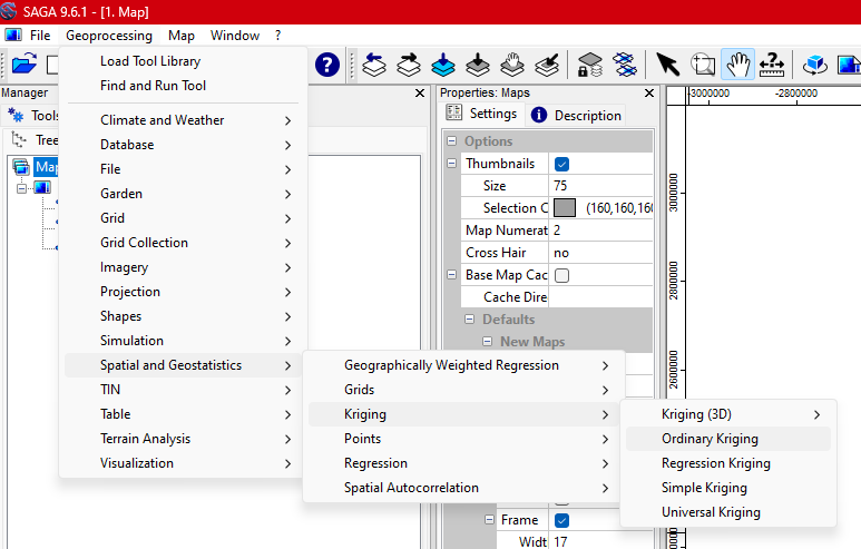
* Navigate to '''''Spatial and Geostatistics''''' → '''''Kriging''''' → '''''Ordinary Kriging'''''. (''Figure 5'' demonstrates this step.) |
|||
::[[Image:SAGApic5.png|thumb|none|frame|1000px|''Figure 5: Kriging Tool Path'']] |
|||
<br> |
|||
'''Step 4: Adjust Kriging Settings''' |
|||
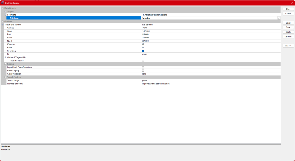
* Use the default Kriging settings for your initial analysis. (''Figure 6'' shows these settings.'') |
|||
* For extended boundaries, customize the settings as needed. In this case we are expanding the boundaries so the interpolated area covers all of Alberta (''Refer to Figure 7 for details.'') |
|||
** ''Extended boundaries are a preferred option as they give a better result.'' |
|||
::[[Image:SAGApic6.png|thumb|none|frame|1000px|''Figure 6: Default Kriging Extent'']] |
|||
::[[Image:SAGApic7.png|thumb|none|frame|1000px|''Figure 7: Expanded Extent'']] |
|||
<br> |
|||
'''Step 5: Variogram''' |
|||
<br> |
|||
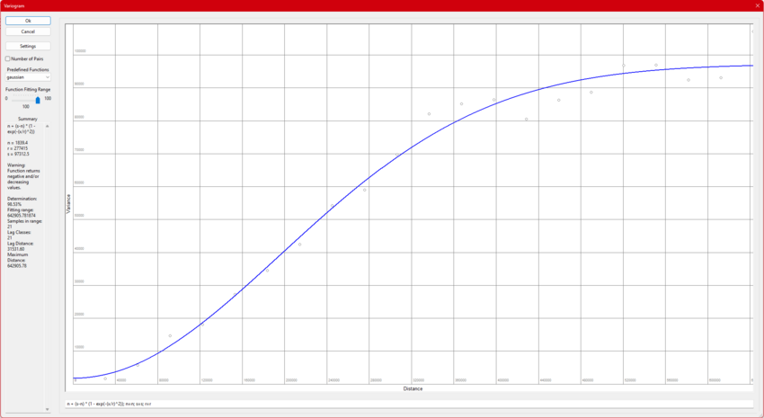
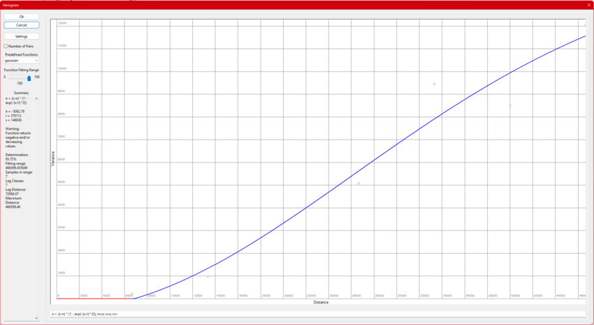
Variograms help in modeling spatial patterns by describing how the variance of data values varies with distance. Because it directly affects the accuracy of Kriging predictions, choosing the variogram with the best determination (best fit to your data) is essential. By reducing interpolation mistakes and guaranteeing that the model appropriately depicts spatial relationships, a well-fitted variogram improves the dependability of your results. Poor variogram selection can lead to biased predictions or the underestimation of variability. |
|||
<br> |
|||
* In the case of this tutorial, both datasets used 100 for the Function Fitting Range. |
|||
** This could cause issues with overfit noise or irrelevant patterns, leading to inaccurate predictions. Please take the time to find the best-fitting range for your data. |
|||
* Both data models also used Gaussian Predefined Functions. |
|||
** This function had the best fit (Determination) with the data used. |
|||
<br> |
|||
* Once this process is completed press '''Ok''' |
|||
<br> |
|||
<div style="display: flex; justify-content: center; gap: 10px"> |
|||
<div style="text-align: center;"> |
|||
[[Image:VariogramAll.png|thumb|none|frame|850px|''Variogram All Weather Stations'']] |
|||
</div> |
|||
<div style="text-align: center;"> |
|||
[[Image:VariogramLimited.png|thumb|none|frame|850px|''Variogram Limited Weather Stations'']] |
|||
</div> |
|||
</div> |
|||
<br> |
|||
'''Step 6: Save Kriging Results''' |
|||
* After completing the Kriging analysis, locate the results in the '''''Data''''' tab under '''''Grids'''''. |
|||
* Rename the result to something meaningful, e.g., "Kriging Analysis". |
|||
(''Figures 9 and 10'' display this process.) |
|||
::[[Image:SAGApic9.png|thumb|none|frame|1000px|''Figure 9: Kriging Result location'']] |
|||
::[[Image:SAGApic10.png|thumb|none|frame|1000px|''Figure 10: Kriging Result Change name'']] |
|||
<br> |
|||
'''Step 7: Clip the Kriging Results''' |
|||
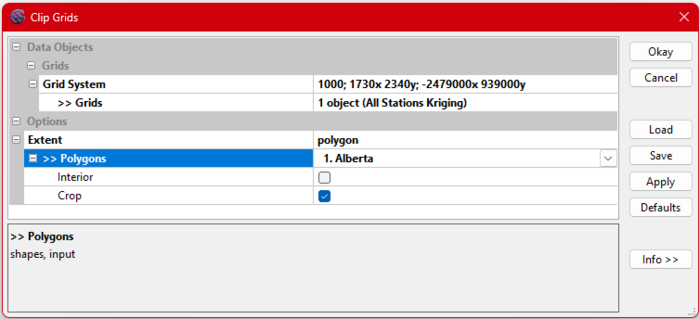
* Go to '''''Geoprocessing''''' → '''''Grid''''' → '''''Grid System''''' → '''''Clip Grids'''''. (''Figure 11'' shows this menu.) |
|||
* Select the appropriate grid system. |
|||
* Use the polygon selection tool to clip the data to the Alberta region: |
|||
** Choose the dotted grid selection. |
|||
** Use the three dots and two arrows tool to define the clip area. |
|||
** Specify Alberta as the clipping region. |
|||
(Refer to ''Figures 11-15'' for guidance.) |
|||
::[[Image:SAGApic11.png|thumb|none|frame|900px|''Figure 11: Path to Clip Tool'']] |
|||
::[[Image:SAGApic12.png|thumb|none|frame|700px|''Figure 12: Selecting the Correct Grid System'']] |
|||
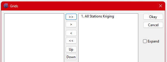
::[[Image:SAGApic13.png|thumb|none|frame|700px|''Figure 13: Clicking on the 3 dots to Select a Grid'']] |
|||
::[[Image:SAGApic14.png|thumb|none|frame|1000px|''Figure 14: Moving the Correct Grid to the Right'']] |
|||
::[[Image:SAGApic15.png|thumb|none|frame|700px|''Figure 15: Selecting the Alberta Polygon to Clip the Grid'']] |
|||
<br> |
|||
'''Step 8: Rename Clipped Results''' |
|||
* Rename the clipped Kriging results to differentiate them from the original dataset. |
|||
* Update the map view to reflect these changes. |
|||
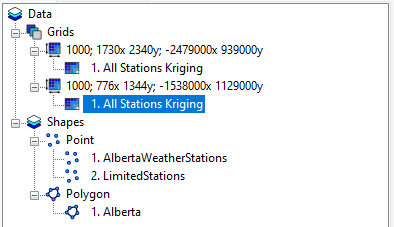
(''Figures 16'' demonstrate this step.) |
|||
::[[Image:SAGApic16.png|thumb|none|frame|1000px|''Figure 16: Rename Clipped Results'']] |
|||
<br> |
|||
'''Step 9: Repeat for Limited Weather Station Data''' |
|||
* Repeat the Kriging analysis and clipping process, this time using data from a limited number of weather stations. |
|||
* Ensure the same steps are followed to maintain consistency. |
|||
'''''Go back to Step 3 and repeat using limited weather stations data.''''' |
|||
<br> |
|||
<br> |
|||
='''Results'''= |
|||
===Visual Comparisons=== |
|||
<div style="display: flex; justify-content: center; gap: 10px"> |
|||
<div style="text-align: center;"> |
|||
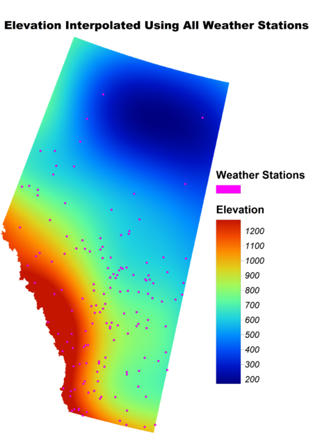
[[Image:SAGAfullmap.png|thumb|none|frame|Elevation Interpolated from all Weather Stations (m)|450px]] |
|||
</div> |
|||
<div style="text-align: center;"> |
|||
[[Image:SAGAlimitedmap.png|thumb|none|frame|Elevation Interpolated from Limited Weather Stations (m)|450px]] |
|||
</div> |
|||
<div style="text-align: center;"> |
|||
[[Image:AlbertaDEM2.png|thumb|none|frame|Alberta Digital Elevation Model (m)|450px]] |
|||
</div> |
|||
</div> |
|||
===Comparing the Accuracy of the Interpolations=== |
|||
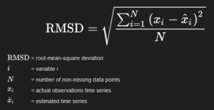
The Root Mean Square Error (RMSE) is a common metric used to quantify the differences between the observed and predicted values, calculated using the formula |
|||
::[[Image:rmse.png|thumb|none|frame|RMSE Formula]] |
|||
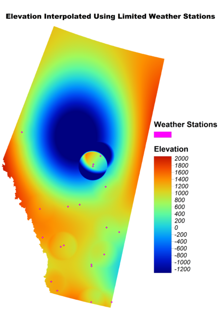
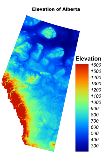
The comparison of the two interpolated results highlights the importance of data quality and quantity in achieving accurate models. Using all available weather station data, the interpolation yielded a root mean square error (RMSE) of 243, demonstrating a high level of accuracy. This result stands in contrast to the interpolation performed with a limited dataset, which resulted in a significantly higher RMSE of 933. The higher error shows substantial inaccuracies and deviations from the actual topography when fewer data points are used. On average, the interpolation using the complete dataset is four times more accurate. Furthermore, this interpolation utilized more than six times the number of data points compared to the limited dataset. |
|||
='''Conclusion'''= |
|||
In this tutorial we used elevation data from Alberta's weather stations in comparison to a subset of 20 random weather stations in the province to illustrate how to do Kriging in SAGA GIS. As well as, examine the effect of data density on the produced elevation surfaces by using the Kriging interpolation method on both datasets. The findings demonstrated that while a smaller selection offers a quicker, but less thorough, analysis, a larger dataset yields a smoother and more detailed interpolation. |
|||
The tutorial underlines the importance of understanding the dataset characteristics and their influence on interpolation results. Using SAGA's built in Kriging tools, the user can make decisions about spatial data sampling and processing to meet the specific needs of their project. |
|||
<br> |
|||
=== Contributions to this tutorial === |
|||
Leo and myself hope that the tutorial continues to evolve as there is much more to kriging than meets the eye and SAGA seems to be a good tool with more to dig into. We thought a few things could be looked at further and could be a starting point for either updating this tutorial or a secondary tutorial. |
|||
<br> |
|||
* Function Fitting Range and the various predefined functions in the variogram section |
|||
**We quickly skimmed over this section of the tutorial, only taking into consideration best fit (determination) when looking at the multiple predefined functions. We also simply used 100 as the Function Fitting Range which can lead to some issues based on overfit noise and irrelevant patterns. |
|||
* Displaying how to run the comparison using either SAGA or another free open-source program. |
|||
**In our tutorial, we displayed the differences and ran a tool but did not incorporate it in the tutorial. This could be a good starting point for a future tutorial or could be added to this one if wanted. |
|||
=== About === |
|||
This tutorial was created in Fall 2024 for GEOM 4008 which is part of the Geomatics program at Carleton University, located in Ottawa, Ontario, Canada, and shows the user how to perform Kriging Interpolation using SAGA GIS on Windows. |
|||
===References=== |
|||
* SAGA GIS - Conrad, O., Bechtel, B., Bock, M., Dietrich, H., Fischer, E., Gerlitz, L., Wehberg, J., Wichmann, V., and Böhner, J. (2015): System for Automated Geoscientific Analyses (SAGA) v. 2.1.4, Geosci. Model Dev., 8, 1991-2007, doi:10.5194/gmd-8-1991-2015. https://gmd.copernicus.org/articles/8/1991/2015/gmd-8-1991-2015.html |
|||
* SAGA GIS Wiki. https://sourceforge.net/p/saga-gis/wiki/Home/ |
|||
*S AGA GIS Tool Ordinary Kriging. https://saga-gis.sourceforge.io/saga_tool_doc/9.0.0/statistics_kriging_0.html |
|||
'''Data'''<br> |
|||
=Tutorial= |
|||
* SAGA GIS software download. https://sourceforge.net/projects/saga-gis/ |
|||
* Access to modified data used in tutorial. [https://drive.google.com/drive/folders/10vHdF1R7j88iQ2xJ6KoINM0LUkJsvLiq?usp=sharing https://drive.google.com/drive/folders/] |
|||
* Weather Station Data. [https://geo1.scholarsportal.info/#_lang=en https://geo1.scholarsportal.info/] |
|||
* Alberta Boundary File. [https://open.canada.ca/data/en/dataset/a883eb14-0c0e-45c4-b8c4-b54c4a819edb/resource/12c03de6-c3f7-4f5f-bb5c-d479f2332842 https://open.canada.ca/data/en/dataset/] |
|||
* Alberta 25M Digital Elevation Model. [https://www.altalis.com/map;id=150 https://www.altalis.com/map] |
|||
<br> |
|||
<br> |
|||
Latest revision as of 13:18, 2 January 2025
Kriging Interpolation Comparison on Alberta Weather Station Elevation Data using System for Automated Geoscientific Analysis (SAGA GIS)
Contents
Introduction
Purpose
The purpose of this tutorial is to provide a step-by-step guide to using the Kriging interpolation technique in SAGA GIS, a software that many users may not have encountered before. The tutorial will introduce the various types of Kriging and the key variables to consider during the process. By comparing results from a dataset with dense data points to one with sparse data, the tutorial aims to highlight the critical role that data quality and quantity play in achieving accurate interpolation results.
Introduction to SAGA
SAGA, short for System for Automated Geoscientific Analyses, is a powerful Geographic Information System (GIS) software designed for the effective implementation of spatial algorithms. It offers a comprehensive and ever-growing suite of geoscientific methods, coupled with an approachable user interface featuring diverse visualization options. SAGA runs on both Windows and Linux operating systems and is distributed as Free Open Source Software (FOSS).
Downloading SAGA
Before beginning the tutorial, if you do not have SAGA GIS please follow the steps below:
- Follow this link to download [1]
- Once the download is complete extract the files from the zip folder
- Run the saga_gui.exe to open the program
Data
Transformed Data used in tutorial is available in the Download Tutorial Data section
Acquiring the Data
To download the Elevation data follow these steps:
- Visit the Scholars GeoPortal.
- In the search bar enter Weather Stations .
- The Canadian Weather Stations should be available to Add to map.
- After adding the data to the map it is possible to select an area. In our case we selected All of Alberta's data.
- Once this is completed, go to the Download page and either download your selected area or the entire dataset.
To download the Alberta boundary file follow these steps:
- Visit the Open Canada
- Download the Provinces/Territories, Cartographic Boundary File - 2016 Census
- Clip to only Alberta or Province of choice. (Clipped Data Available In Download Tutorial Data Section)
To download the Alberta 25M Digital Elevation Model follow these steps:
- Go to Altalis.com
- Create Altalis account to download the free 25M Digital Elevation Model
- Add the 25M Raster DEM to your cart.
- Go to cart and Proceed with Download.
- An email with your file ready to download will be sent to you shortly.
Download Tutorial Data
All the data and code can be downloaded from this Google Drive Link
The download contains:
TutorialDataDownload.zip (124KB)
- Alberta Boundary Shapefile (152KB) [1]
- Alberta Weather Station Data (100KB) [2]
- Limited Alberta Weather Station Data (30.4KB) [3]
AlbertaDEM.zip(1.18GB) *Optional
- Alberta 25M Digital Elevation Model (8.25GB) [4]
Tutorial
SAGA GIS Interpolation Options
Saga has four different types of interpolation, each with their own strengths, weaknesses and specific characterstics. We will explain the use cases of each of them. They also have a 3D Kriging tool that we will not go into detail in this tutorial. There are also lots of different options and inputs that modify the kriging in SAGA which we will explain and how they impact the interpolation.
- Ordinary Kriging
- Assumptions: Assumes the mean of the data is unknown but constant over the area of interest.
- Advantages: Simple, widely applicable, and does not require external data or a predefined trend.
- Use Case: Best for spatially autocorrelated data with no obvious trends or external influencing factors.
- Regression Kriging
- Assumptions: Combines a deterministic regression model with kriging of residuals.
- Advantages: Incorporates additional explanatory variables (e.g., slope, aspect) to improve accuracy.
- Use Case: Ideal when auxiliary data strongly influences the spatial distribution of the variable.
- Simple Kriging
- Assumptions: Assumes a known and constant mean across the study area.
- Advantages: Computationally efficient and straightforward but requires prior knowledge of the mean.
- Use Case: Rarely used unless the mean is well-established (e.g., synthetic datasets).
- Universal Kriging
- Assumptions: Assumes the data has a deterministic trend (e.g., polynomial or linear) over space.
- Advantages: Models and accounts for spatial trends while still relying on kriging for local variation.
- Use Case: Useful for non-stationary data with a noticeable trend (e.g., elevation gradients across a region).
Kriging Interpolation Step-By-Step
Step 1: Open the Data Files
- Navigate to File → Open.
- Open each data file individually. (the files with .shp file format)
- Ensure all the data has been added correctly. Go to the Manager tab → Data → Tree
Step 2: Add Files to the Map
- Right-click on each file and select Add to Map.
- Ensure that all files are added to the same map. Avoid creating separate maps for each file. ( See Figure 2 through 4 for the exact steps and expected outcome.)
Step 3: Kriging Analysis Setup
- Go to Geoprocessing tab.
- Navigate to Spatial and Geostatistics → Kriging → Ordinary Kriging. (Figure 5 demonstrates this step.)
Step 4: Adjust Kriging Settings
- Use the default Kriging settings for your initial analysis. (Figure 6 shows these settings.)
- For extended boundaries, customize the settings as needed. In this case we are expanding the boundaries so the interpolated area covers all of Alberta (Refer to Figure 7 for details.)
- Extended boundaries are a preferred option as they give a better result.
Step 5: Variogram
Variograms help in modeling spatial patterns by describing how the variance of data values varies with distance. Because it directly affects the accuracy of Kriging predictions, choosing the variogram with the best determination (best fit to your data) is essential. By reducing interpolation mistakes and guaranteeing that the model appropriately depicts spatial relationships, a well-fitted variogram improves the dependability of your results. Poor variogram selection can lead to biased predictions or the underestimation of variability.
- In the case of this tutorial, both datasets used 100 for the Function Fitting Range.
- This could cause issues with overfit noise or irrelevant patterns, leading to inaccurate predictions. Please take the time to find the best-fitting range for your data.
- Both data models also used Gaussian Predefined Functions.
- This function had the best fit (Determination) with the data used.
- Once this process is completed press Ok
Step 6: Save Kriging Results
- After completing the Kriging analysis, locate the results in the Data tab under Grids.
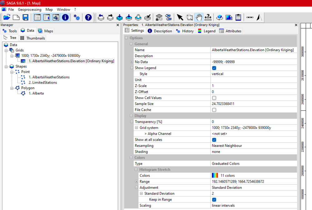
- Rename the result to something meaningful, e.g., "Kriging Analysis".
(Figures 9 and 10 display this process.)
Step 7: Clip the Kriging Results
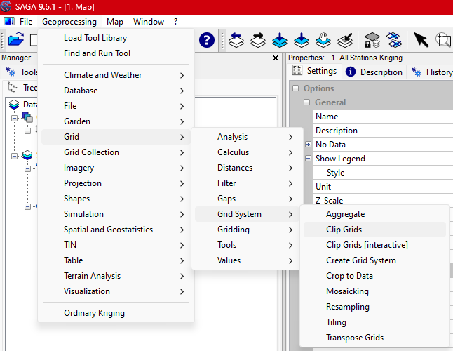
- Go to Geoprocessing → Grid → Grid System → Clip Grids. (Figure 11 shows this menu.)
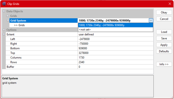
- Select the appropriate grid system.
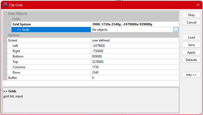
- Use the polygon selection tool to clip the data to the Alberta region:
- Choose the dotted grid selection.
- Use the three dots and two arrows tool to define the clip area.
- Specify Alberta as the clipping region.
(Refer to Figures 11-15 for guidance.)
Step 8: Rename Clipped Results
- Rename the clipped Kriging results to differentiate them from the original dataset.
- Update the map view to reflect these changes.
(Figures 16 demonstrate this step.)
Step 9: Repeat for Limited Weather Station Data
- Repeat the Kriging analysis and clipping process, this time using data from a limited number of weather stations.
- Ensure the same steps are followed to maintain consistency.
Go back to Step 3 and repeat using limited weather stations data.
Results
Visual Comparisons
Comparing the Accuracy of the Interpolations
The Root Mean Square Error (RMSE) is a common metric used to quantify the differences between the observed and predicted values, calculated using the formula
The comparison of the two interpolated results highlights the importance of data quality and quantity in achieving accurate models. Using all available weather station data, the interpolation yielded a root mean square error (RMSE) of 243, demonstrating a high level of accuracy. This result stands in contrast to the interpolation performed with a limited dataset, which resulted in a significantly higher RMSE of 933. The higher error shows substantial inaccuracies and deviations from the actual topography when fewer data points are used. On average, the interpolation using the complete dataset is four times more accurate. Furthermore, this interpolation utilized more than six times the number of data points compared to the limited dataset.
Conclusion
In this tutorial we used elevation data from Alberta's weather stations in comparison to a subset of 20 random weather stations in the province to illustrate how to do Kriging in SAGA GIS. As well as, examine the effect of data density on the produced elevation surfaces by using the Kriging interpolation method on both datasets. The findings demonstrated that while a smaller selection offers a quicker, but less thorough, analysis, a larger dataset yields a smoother and more detailed interpolation.
The tutorial underlines the importance of understanding the dataset characteristics and their influence on interpolation results. Using SAGA's built in Kriging tools, the user can make decisions about spatial data sampling and processing to meet the specific needs of their project.
Contributions to this tutorial
Leo and myself hope that the tutorial continues to evolve as there is much more to kriging than meets the eye and SAGA seems to be a good tool with more to dig into. We thought a few things could be looked at further and could be a starting point for either updating this tutorial or a secondary tutorial.
- Function Fitting Range and the various predefined functions in the variogram section
- We quickly skimmed over this section of the tutorial, only taking into consideration best fit (determination) when looking at the multiple predefined functions. We also simply used 100 as the Function Fitting Range which can lead to some issues based on overfit noise and irrelevant patterns.
- Displaying how to run the comparison using either SAGA or another free open-source program.
- In our tutorial, we displayed the differences and ran a tool but did not incorporate it in the tutorial. This could be a good starting point for a future tutorial or could be added to this one if wanted.
About
This tutorial was created in Fall 2024 for GEOM 4008 which is part of the Geomatics program at Carleton University, located in Ottawa, Ontario, Canada, and shows the user how to perform Kriging Interpolation using SAGA GIS on Windows.
References
- SAGA GIS - Conrad, O., Bechtel, B., Bock, M., Dietrich, H., Fischer, E., Gerlitz, L., Wehberg, J., Wichmann, V., and Böhner, J. (2015): System for Automated Geoscientific Analyses (SAGA) v. 2.1.4, Geosci. Model Dev., 8, 1991-2007, doi:10.5194/gmd-8-1991-2015. https://gmd.copernicus.org/articles/8/1991/2015/gmd-8-1991-2015.html
- SAGA GIS Wiki. https://sourceforge.net/p/saga-gis/wiki/Home/
- S AGA GIS Tool Ordinary Kriging. https://saga-gis.sourceforge.io/saga_tool_doc/9.0.0/statistics_kriging_0.html
Data
- SAGA GIS software download. https://sourceforge.net/projects/saga-gis/
- Access to modified data used in tutorial. https://drive.google.com/drive/folders/
- Weather Station Data. https://geo1.scholarsportal.info/
- Alberta Boundary File. https://open.canada.ca/data/en/dataset/
- Alberta 25M Digital Elevation Model. https://www.altalis.com/map
