Difference between revisions of "Glacier Change Detection in GRASS GIS"
OwenKirkham (talk | contribs) |
|||
| (10 intermediate revisions by one other user not shown) | |||
| Line 1: | Line 1: | ||
== |
== Introduction == |
||
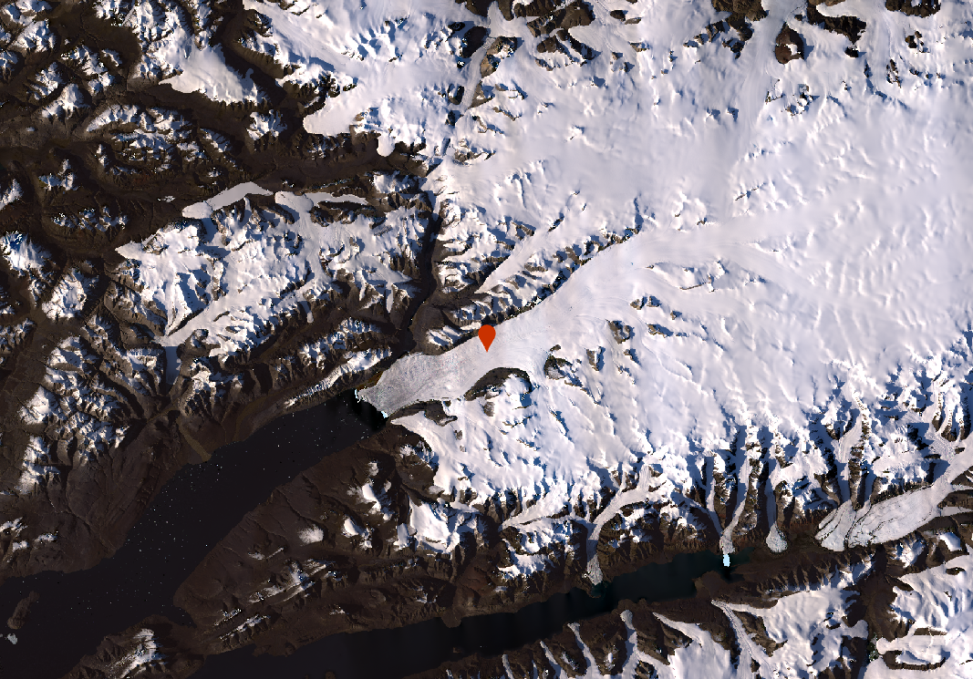
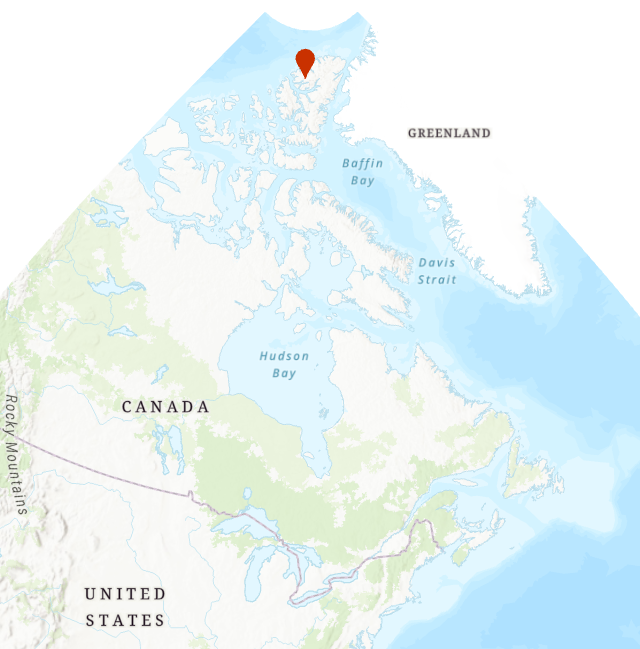
This tutorial will use Grass GIS to perform a change detection analysis on Landsat imagery of the Otto Glacier, a marine-terminating glacier located on Ellesmere Island in Nunavut. Ellesmere Island's mean annual air temperature has increased by 3.6°C between 1948 and 2016, reducing ice coverage by 3.68% in the last decade (White & Copland, 2018). The tutorial demonstrated how to visualize and quantify recent changes in the Otto glacier while demonstrating key GIS concepts such as the Normalized Difference Snow Index (NDSI), raster math, raster clipping, and raster visualization within Grass GIS. |
|||
[[File:OttoGlacier.PNG]] |
|||
== Introduction == |
|||
[[File:Inset.PNG]] |
|||
== Software Download and Instillation == |
== Software Download and Instillation == |
||
| Line 22: | Line 24: | ||
{| class="wikitable" |
{| class="wikitable" |
||
|- |
|- |
||
! Landsat Image ID !! |
! Year !! Landsat Image ID !! Name of images |
||
|- |
|- |
||
| 2014 || LC08_L2SP_060246_20140825_20200911_02_T1 || L8_20140825_B3, L8_20140825_B6 |
|||
| LC08_L2SP_060246_20140825_20200911_02_T1 || Example || Example |
|||
|- |
|- |
||
| 2015 || LC08_L2SP_046248_20150810_20200908_02_T1 || LC08_L2SP_046248_20150810_20200908_02_T1_SR_B3, LC08_L2SP_046248_20150810_20200908_02_T1_SR_B6 |
|||
| LC08_L2SP_046248_20150810_20200908_02_T1 || Example || Example |
|||
|- |
|- |
||
| 2016 || LC08_L2SP_057001_20160825_20200906_02_T1 || LC08_L2SP_057001_20160825_20200906_02_T1_SR_B3, LC08_L2SP_057001_20160825_20200906_02_T1_SR_B6 |
|||
| LC08_L2SP_057001_20160825_20200906_02_T1 || Example || Example |
|||
|- |
|- |
||
| 2018 || LC08_L2SP_046248_20180802_20200831_02_T1 || LC08_L2SP_046248_20180802_20200831_02_T1_SR_B3, LC08_L2SP_046248_20180802_20200831_02_T1_SR_B6 |
|||
| LC08_L2SP_046248_20180802_20200831_02_T1 || Example || Example |
|||
|- |
|- |
||
| 2019 || LC08_L2SP_048248_20190718_20200827_02_T1 || L8_20190718_B3, L820190718_B6 |
|||
| LC08_L2SP_048248_20190718_20200827_02_T1 || Example || Example |
|||
|- |
|- |
||
| 2020 || LC08_L2SP_074244_20200811_20200918_02_T1 || L8_20200811_B3, L8_20200811_B6 |
|||
| LC08_L2SP_074244_20200811_20200918_02_T1 || Example || Example |
|||
|- |
|- |
||
| 2022 || LC09_L2SP_046248_20220821_20230401_02_T1 || LC09_L2SP_046248_20220821_20230401_02_T1_SR_B3, LC09_L2SP_046248_20220821_20230401_02_T1_SR_B6 |
|||
| LC09_L2SP_046248_20220821_20230401_02_T1 || Example || Example |
|||
|- |
|- |
||
| 2023 || LC08_L2SP_067245_20230819_20230826_02_T1 || L8_20230819_B3, L8_20230819_B6 |
|||
| LC08_L2SP_067245_20230819_20230826_02_T1 || Example || Example |
|||
|- |
|- |
||
| 2024 || LC09_L2SP_052247_20240820_20240821_02_T1 || LC09_L2SP_052247_20240820_20240821_02_T1_SR_B3, LC09_L2SP_052247_20240820_20240821_02_T1_SR_B6 |
|||
| LC09_L2SP_052247_20240820_20240821_02_T1 || Example || Example |
|||
|} |
|} |
||
| Line 49: | Line 51: | ||
== Methods == |
== Methods == |
||
=== Set Up === |
=== Set Up Project=== |
||
Open GRASS GIS |
|||
Press the "Create new project" button [[File:Projectbutton.PNG]] |
|||
Give the project a relevant name, such as ChangeDetection or GlacierChangeDetection. Press "Next" |
|||
[[File:Newproject.PNG]] |
|||
Then, select "Select CRS from a list by EPSG or description." Press "Next" |
|||
[[File:Project2.PNG]] |
|||
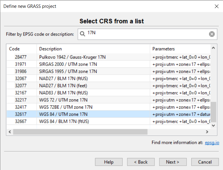
Next, type "17N" into the search bar and scroll down until you find the "WGS 84 / UTM zone 17N" projection. Press "Next" |
|||
[[File:Project3.PNG]] |
|||
Finally, press "Finish" |
|||
=== Import Raster Data === |
=== Import Raster Data === |
||
Landsat imagery from USGS Earth Explorer will |
Landsat imagery from USGS Earth Explorer will be downloaded in a TAR format. Use the 7Zip file manager to extract the. TIF files. |
||
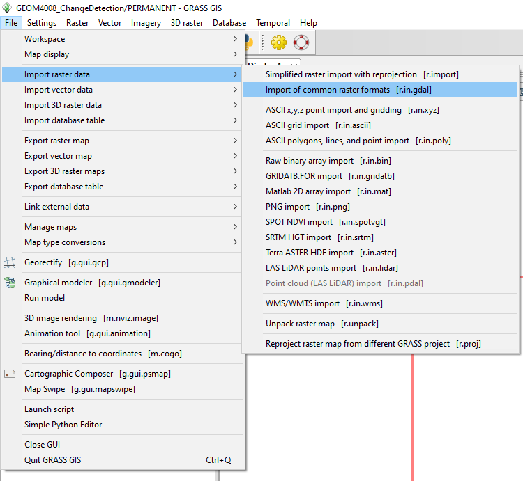
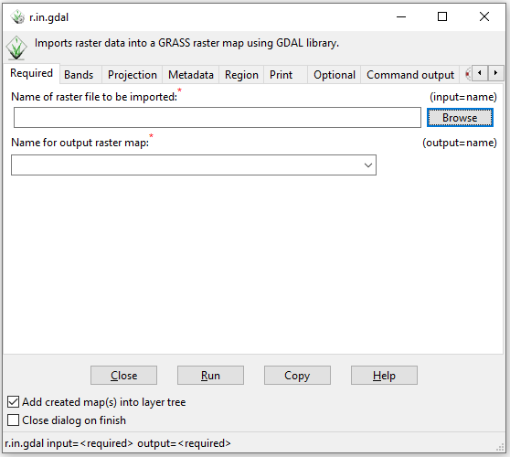
To import the Landsat images to the workspace, go to "File" > "Import raster data" > "Import of common raster formats [r.in.gdal]" |
To import the Landsat images to the workspace, go to "File" > "Import raster data" > "Import of common raster formats [r.in.gdal]" |
||
| Line 60: | Line 79: | ||
[[File:Add rasters.png]] |
[[File:Add rasters.png]] |
||
Next, press "Browse" and find the extracted folders for the Landsat imagery. |
Next, press "Browse" and find the extracted folders for the Landsat imagery. For each image, import bands 3 and 6 (TIF files ending in "B6" and "B3"). To make the analysis easier, use a standardized naming convention for all of the images. For example, bands 3 and 6 from the 2014 image can be named L8_2014_B3 and L8_2014_B6, respectively. |
||
=== Import Vector Data === |
=== Import Vector Data === |
||
To import the computation region and Otto Glacier outline vector files, go to "File" > "Import vector data" > "Import of common vector formats [v.in.ogr]". |
To import the computation region and Otto Glacier outline vector files, go to "File" > "Import vector data" > "Import of common vector formats [v.in.ogr]". |
||
Using the "Browse" button, find the "CR.shp" and "OttoFiord17N.shp" shapefiles that were downloaded earlier |
Using the "Browse" button, find the "CR.shp" and "OttoFiord17N.shp" shapefiles that were downloaded earlier and import them one at a time. |
||
[[File:Add rasters 2.PNG]] |
[[File:Add rasters 2.PNG]] |
||
| Line 71: | Line 90: | ||
=== Set Computational Region === |
=== Set Computational Region === |
||
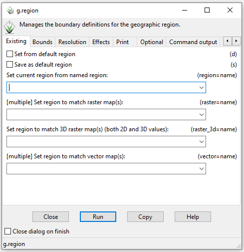
GRASS GIS requires a computational region to |
GRASS GIS requires a computational region to perform calculations on a raster properly. To set the computational region, "Settings" > "Computational region" > "Set region [g.region]". |
||
Find the drop-down menu called "[multiple] Set |
Find the drop-down menu called "[multiple] Set regions to match vector map(s)," and select the "CR" vector layer—press run. |
||
[[File:Set_region_2.PNG]] |
[[File:Set_region_2.PNG]] |
||
| Line 79: | Line 98: | ||
=== Mask Rasters === |
=== Mask Rasters === |
||
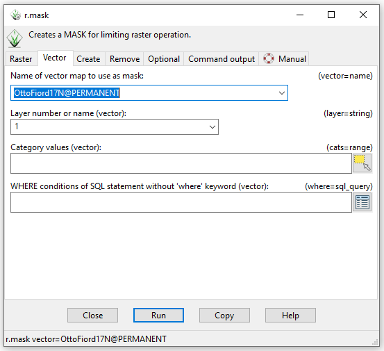
We will use a vector mask to mask the Landsat imagery to isolate the glacier tongue from the rest of the image. |
|||
To isolate the glacier tongue from the rest of the image, we will use a vector mask tp mask the Landsat imagery. |
|||
To create a mask, go to "Raster" > "Mask [r.mask] |
To create a mask, go to "Raster" > "Mask [r.mask]." Then, press on the "Vector" tab and select "OttoFiord17N" from the "Name of vector map to use as a mask" drop-down menu—press run. |
||
[[File:Mask.PNG]] |
[[File:Mask.PNG]] |
||
| Line 95: | Line 114: | ||
The NDSI formula is "(Green-SWIR)/(Green+SWIR)," where Green is the green band, and SWIR is the SWIR band for an image. For Landsat 8/9 imagery, B3 is the green band, and B6 is the SWIR band. |
The NDSI formula is "(Green-SWIR)/(Green+SWIR)," where Green is the green band, and SWIR is the SWIR band for an image. For Landsat 8/9 imagery, B3 is the green band, and B6 is the SWIR band. |
||
In the "Expression" text box, paste this formula: '''(float( raster_B3 ) - float( raster_B6 ) ) /(float( raster_B3 ) + float( raster_B6 ) )'''. The float function allows the output to have decimal places. |
In the "Expression" text box, paste this formula: '''(float( raster_B3 ) - float( raster_B6 ) ) /(float( raster_B3 ) + float( raster_B6 ) )'''. The float function allows the output to have decimal places; without specifying that, the default would be to write integer results since that was the format of the input data layers. |
||
Then, change raster_B3 and raster_B6 to the appropriate names. Raster names can be input by clicking |
Then, change raster_B3 and raster_B6 to the appropriate names. Raster names can be input by clicking the raster from the "Insert existing raster map" drop-down menu. |
||
Finally, press "Run". The new NDSI raster will be added to the workspace. Repeat this step for every Landsat image in the time series. |
Finally, press "Run". The new NDSI raster will be added to the workspace. Repeat this step for every Landsat image in the time series. |
||
| Line 105: | Line 124: | ||
=== Convert Null values === |
=== Convert Null values === |
||
The rasters contain Null values that will hinder the analysis. To |
The rasters contain Null values that will hinder the analysis. To address this problem, we will set the null values to 0. |
||
First, go to "Rasters" > "Develop raster map" > "Manage Null values [r.null]" |
First, go to "Rasters" > "Develop raster map" > "Manage Null values [r.null]" |
||
| Line 111: | Line 130: | ||
[[File:Null.png]] |
[[File:Null.png]] |
||
Then, |
Then, in the "Name of raster map" drop-down menu, change the input raster to an NDVI raster. |
||
Next, go to the "Modify" tab and enter 0 in the "The value to replace the null value by" box. Press run and repeat for all of the NDSI rasters. |
Next, go to the "Modify" tab and enter 0 in the "The value to replace the null value by" box. Press run and repeat for all of the NDSI rasters. |
||
| Line 119: | Line 138: | ||
=== Reclassify NDSI Rasters === |
=== Reclassify NDSI Rasters === |
||
Once we calculate the NDSI rasters, we |
Once we calculate the NDSI rasters, we must reclassify them to identify the glacier from the rest of the image. The NDSI rasters have values between -1 and 1, with values greater than 0.4 representing snow or ice. |
||
Open the raster calculator. In the expression box, paste this formula: ```if ( NDSI_raster >= 0.4, 1, if( NDSI_raster < 0.4,0))```, and change the name from "NDSI_raster" to the name of the 2014 raster. |
Open the raster calculator. In the expression box, paste this formula: ```if ( NDSI_raster >= 0.4, 1, if( NDSI_raster < 0.4,0))```, and change the name from "NDSI_raster" to the name of the 2014 raster. |
||
| Line 141: | Line 160: | ||
Next, input the name of the 2014 reclassified NDSI raster into the "Name of input raster map" box. Name the output vector layer "Extent2014", and change the "Output feature type" to "area". Press run |
Next, input the name of the 2014 reclassified NDSI raster into the "Name of input raster map" box. Name the output vector layer "Extent2014", and change the "Output feature type" to "area". Press run |
||
This tool's output will be a vector of the 2014 NDSI reclassified raster with values of 1 and 0. |
|||
[[File:Convert_2.PNG]] |
[[File:Convert_2.PNG]] |
||
Then, with the Extent2014 layer displayed on the map, press the select feature's icon |
Then, with the Extent2014 layer displayed on the map, press the select feature's icon and press on the glacier polygon within the layer. The selection should look like this: |
||
[[File:Convert_3.png]] |
[[File:Convert_3.png]] |
||
| Line 153: | Line 172: | ||
=== Time Series Change Detection with Landsat 8/9=== |
=== Time Series Change Detection with Landsat 8/9=== |
||
The time series change detection has two parts. First, we will visualize the extent of the Otto Glacier Tongue's change over the 10-year time series. Then, we will calculate the change statistics. |
|||
Open the raster map calculator, and paste this expression into the expression box: ```2014_NDSI_Reclass@PERMANENT + 2015_NDSI_Reclass@PERMANENT + 2016_NDSI_Reclass@PERMANENT + 2018_NDSI_Reclass@PERMANENT + 2019_NDSI_Reclass@PERMANENT + 2020_NDSI_Reclass@PERMANENT + 2023_NDSI_Reclass@PERMANENT + 2024_NDSI_Reclass@PERMANENT``` |
Open the raster map calculator, and paste this expression into the expression box: ```2014_NDSI_Reclass@PERMANENT + 2015_NDSI_Reclass@PERMANENT + 2016_NDSI_Reclass@PERMANENT + 2018_NDSI_Reclass@PERMANENT + 2019_NDSI_Reclass@PERMANENT + 2020_NDSI_Reclass@PERMANENT + 2023_NDSI_Reclass@PERMANENT + 2024_NDSI_Reclass@PERMANENT``` |
||
Change the raster names if required, give the output raster a name, and press run |
Change the raster names if required, give the output raster a name, and press run. |
||
[[File:FinalCalc.PNG]] |
[[File:FinalCalc.PNG]] |
||
The final output will have values between 1 and 8. A cell value of 1 represents parts of the glacier tongue that disappeared after 2014, a value of |
The final output will have values between 1 and 8. A cell value of 1 represents parts of the glacier tongue that disappeared after 2014, a value of 2 represents parts of the glacier tongue that disappeared after 2015, a value of three represents parts of the glacier that disappeared after 2016, and so on. Cells with a maximum value of 8 represent the remaining extent of the glacier. |
||
To better visualize this trend, we can change the symbolization of the output raster. |
To better visualize this trend, we can change the symbolization of the output raster. |
||
| Line 171: | Line 190: | ||
The second step of the time series detection is to conduct a simple statistical analysis of the rate and magnitude of change in the glacier tongue. |
The second step of the time series detection is to conduct a simple statistical analysis of the rate and magnitude of change in the glacier tongue. |
||
Go to "Raster" > "Reports and statistics" > "Sum area by raster by raster map and category [r.report]". Select the GlacierChange raster, and check the "area in kilometres under the "Statistics" |
Go to "Raster" > "Reports and statistics" > "Sum area by raster by raster map and category [r.report]". Select the GlacierChange raster, and check the "area in kilometres under the "Statistics" tab—press run. |
||
[[File:Stats_3.PNG]] |
[[File:Stats_3.PNG]] |
||
This tool's output is a statistical report that provides the total area in square kilometres, cell count, and percent cover of each raster class. |
|||
[[File:Stats_2.PNG]] |
[[File:Stats_2.PNG]] |
||
| Line 182: | Line 201: | ||
== Conclusion == |
== Conclusion == |
||
In conclusion, the tutorial teaches users about the impacts of climate change in the Arctic through an informative demonstration of GRASS GIS and universal raster calculator-based raster analysis. Some key concepts demonstrated in this tutorial were raster math, NDSI, raster masking, raster reclassification, and statistical analysis of rasters. |
|||
Latest revision as of 12:08, 3 January 2025
Introduction
This tutorial will use Grass GIS to perform a change detection analysis on Landsat imagery of the Otto Glacier, a marine-terminating glacier located on Ellesmere Island in Nunavut. Ellesmere Island's mean annual air temperature has increased by 3.6°C between 1948 and 2016, reducing ice coverage by 3.68% in the last decade (White & Copland, 2018). The tutorial demonstrated how to visualize and quantify recent changes in the Otto glacier while demonstrating key GIS concepts such as the Normalized Difference Snow Index (NDSI), raster math, raster clipping, and raster visualization within Grass GIS.
Software Download and Instillation
This tutorial is demonstrated in Windows using GRASS GIS version 8.4.0. The latest version of GRASS GIS can be downloaded here
Data Sources
Landsat 8/9 Imagery
This tutorial uses the green and Short-Wave Infrared (SWIR) bands from 8 Landsat 8/9 images. The images were captured in late July/august when the Fiord was mostly free of ice. The Landsat imagery used in this tutorial can be found here
Additional Landsat imagery can be downloaded from the USGS Earth Explorer website. To download the data, create a free student account.
The ID and metadata for the specific images used in this lab are in the table below.
| Year | Landsat Image ID | Name of images |
|---|---|---|
| 2014 | LC08_L2SP_060246_20140825_20200911_02_T1 | L8_20140825_B3, L8_20140825_B6 |
| 2015 | LC08_L2SP_046248_20150810_20200908_02_T1 | LC08_L2SP_046248_20150810_20200908_02_T1_SR_B3, LC08_L2SP_046248_20150810_20200908_02_T1_SR_B6 |
| 2016 | LC08_L2SP_057001_20160825_20200906_02_T1 | LC08_L2SP_057001_20160825_20200906_02_T1_SR_B3, LC08_L2SP_057001_20160825_20200906_02_T1_SR_B6 |
| 2018 | LC08_L2SP_046248_20180802_20200831_02_T1 | LC08_L2SP_046248_20180802_20200831_02_T1_SR_B3, LC08_L2SP_046248_20180802_20200831_02_T1_SR_B6 |
| 2019 | LC08_L2SP_048248_20190718_20200827_02_T1 | L8_20190718_B3, L820190718_B6 |
| 2020 | LC08_L2SP_074244_20200811_20200918_02_T1 | L8_20200811_B3, L8_20200811_B6 |
| 2022 | LC09_L2SP_046248_20220821_20230401_02_T1 | LC09_L2SP_046248_20220821_20230401_02_T1_SR_B3, LC09_L2SP_046248_20220821_20230401_02_T1_SR_B6 |
| 2023 | LC08_L2SP_067245_20230819_20230826_02_T1 | L8_20230819_B3, L8_20230819_B6 |
| 2024 | LC09_L2SP_052247_20240820_20240821_02_T1 | LC09_L2SP_052247_20240820_20240821_02_T1_SR_B3, LC09_L2SP_052247_20240820_20240821_02_T1_SR_B6 |
Supplementary Vector Data
The supplementary vector data for this tutorial can be found here. The vector data includes a polygon computational region and a polygon outline of the Otto Glacier.
Methods
Set Up Project
Open GRASS GIS
Press the "Create new project" button
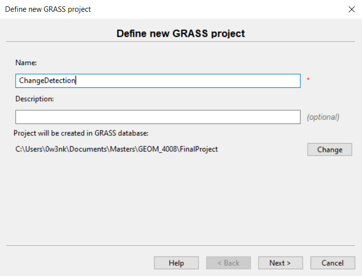
Give the project a relevant name, such as ChangeDetection or GlacierChangeDetection. Press "Next"
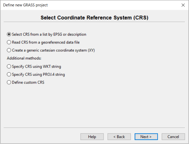
Then, select "Select CRS from a list by EPSG or description." Press "Next"
Next, type "17N" into the search bar and scroll down until you find the "WGS 84 / UTM zone 17N" projection. Press "Next"
Finally, press "Finish"
Import Raster Data
Landsat imagery from USGS Earth Explorer will be downloaded in a TAR format. Use the 7Zip file manager to extract the. TIF files.
To import the Landsat images to the workspace, go to "File" > "Import raster data" > "Import of common raster formats [r.in.gdal]"
Next, press "Browse" and find the extracted folders for the Landsat imagery. For each image, import bands 3 and 6 (TIF files ending in "B6" and "B3"). To make the analysis easier, use a standardized naming convention for all of the images. For example, bands 3 and 6 from the 2014 image can be named L8_2014_B3 and L8_2014_B6, respectively.
Import Vector Data
To import the computation region and Otto Glacier outline vector files, go to "File" > "Import vector data" > "Import of common vector formats [v.in.ogr]".
Using the "Browse" button, find the "CR.shp" and "OttoFiord17N.shp" shapefiles that were downloaded earlier and import them one at a time.
Set Computational Region
GRASS GIS requires a computational region to perform calculations on a raster properly. To set the computational region, "Settings" > "Computational region" > "Set region [g.region]".
Find the drop-down menu called "[multiple] Set regions to match vector map(s)," and select the "CR" vector layer—press run.
Mask Rasters
We will use a vector mask to mask the Landsat imagery to isolate the glacier tongue from the rest of the image.
To create a mask, go to "Raster" > "Mask [r.mask]." Then, press on the "Vector" tab and select "OttoFiord17N" from the "Name of vector map to use as a mask" drop-down menu—press run.
Calculate NDSI
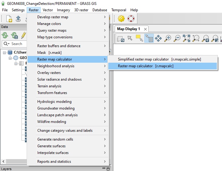
Use the "Raster map calculator" to calculate the NDSI rasters for each year. To find the raster calculator, go to "Raster" > "Raster map calculator" > "Raster map calculator [r.mapcalc]".
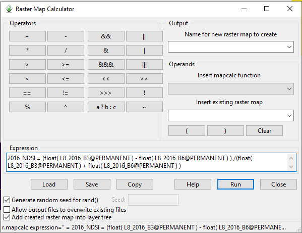
The NDSI formula is "(Green-SWIR)/(Green+SWIR)," where Green is the green band, and SWIR is the SWIR band for an image. For Landsat 8/9 imagery, B3 is the green band, and B6 is the SWIR band.
In the "Expression" text box, paste this formula: (float( raster_B3 ) - float( raster_B6 ) ) /(float( raster_B3 ) + float( raster_B6 ) ). The float function allows the output to have decimal places; without specifying that, the default would be to write integer results since that was the format of the input data layers.
Then, change raster_B3 and raster_B6 to the appropriate names. Raster names can be input by clicking the raster from the "Insert existing raster map" drop-down menu.
Finally, press "Run". The new NDSI raster will be added to the workspace. Repeat this step for every Landsat image in the time series.
Convert Null values
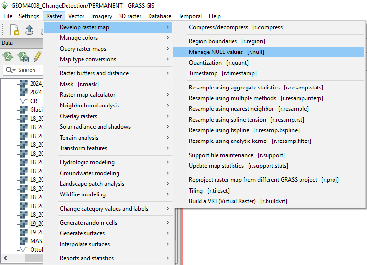
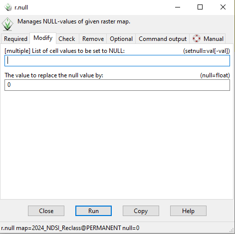
The rasters contain Null values that will hinder the analysis. To address this problem, we will set the null values to 0.
First, go to "Rasters" > "Develop raster map" > "Manage Null values [r.null]"
Then, in the "Name of raster map" drop-down menu, change the input raster to an NDVI raster.
Next, go to the "Modify" tab and enter 0 in the "The value to replace the null value by" box. Press run and repeat for all of the NDSI rasters.
Reclassify NDSI Rasters
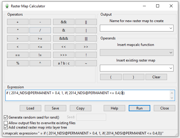
Once we calculate the NDSI rasters, we must reclassify them to identify the glacier from the rest of the image. The NDSI rasters have values between -1 and 1, with values greater than 0.4 representing snow or ice.
Open the raster calculator. In the expression box, paste this formula: ```if ( NDSI_raster >= 0.4, 1, if( NDSI_raster < 0.4,0))```, and change the name from "NDSI_raster" to the name of the 2014 raster.
Press run and repeat with the other 7 NDSI rasters.
This formula tells the raster calculator to reclassify the raster values as 1 if they have an NDSI value greater than 0.4 and 0 if they have a value less than 0.4. Cells with a value of 1 represent the glacier, and cells with a value of 0 represent everything else
Converting Raster to Vector
Before starting the time series analysis, we need to create a new vector mask that describes the maximum extent of the glacier. This will help eliminate noise created by remnant sea ice in the Fiord that was incorrectly identified as the glacier in the NDVI raster.
For this step, we will assume that the 2014 reclassified NDSI raster describes the maximum extent of the glacier within the 10 years of imagery in the time series.
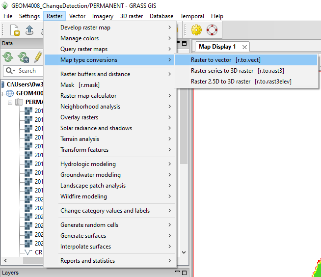
First, go to "Raster" > "Map type conversions" > "Raster to vector [r.to.vect]"
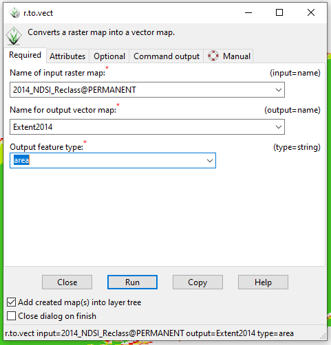
Next, input the name of the 2014 reclassified NDSI raster into the "Name of input raster map" box. Name the output vector layer "Extent2014", and change the "Output feature type" to "area". Press run
This tool's output will be a vector of the 2014 NDSI reclassified raster with values of 1 and 0.
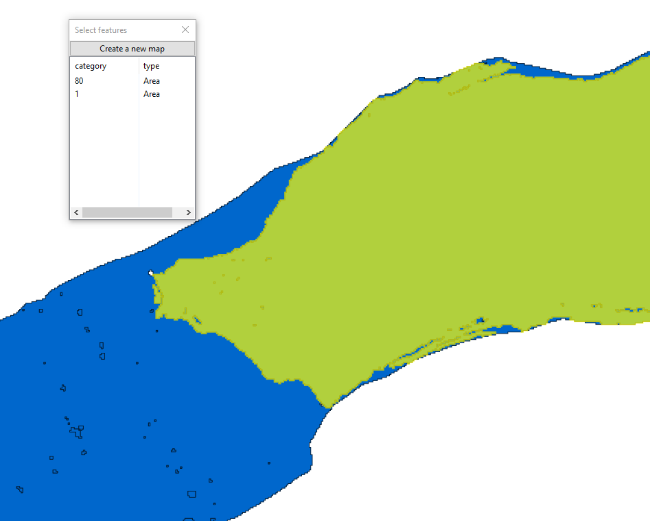
Then, with the Extent2014 layer displayed on the map, press the select feature's icon and press on the glacier polygon within the layer. The selection should look like this:
Finally, press the "Create new map" button to create a new layer. Delete the previous vector mask from the workspace and create a new mask using this Extent2014_selection layer.
Time Series Change Detection with Landsat 8/9
The time series change detection has two parts. First, we will visualize the extent of the Otto Glacier Tongue's change over the 10-year time series. Then, we will calculate the change statistics.
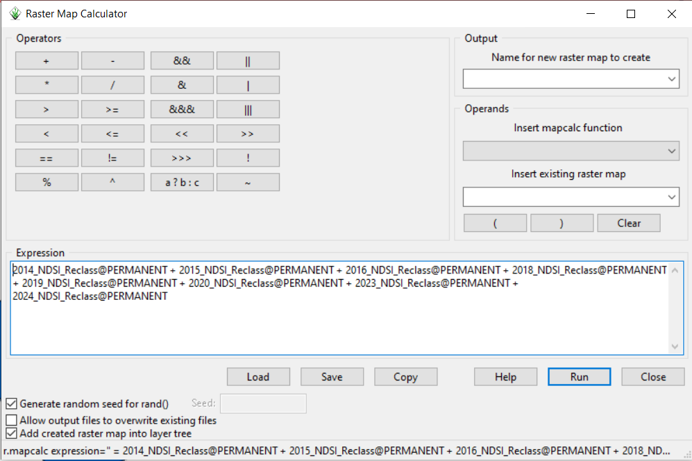
Open the raster map calculator, and paste this expression into the expression box: ```2014_NDSI_Reclass@PERMANENT + 2015_NDSI_Reclass@PERMANENT + 2016_NDSI_Reclass@PERMANENT + 2018_NDSI_Reclass@PERMANENT + 2019_NDSI_Reclass@PERMANENT + 2020_NDSI_Reclass@PERMANENT + 2023_NDSI_Reclass@PERMANENT + 2024_NDSI_Reclass@PERMANENT```
Change the raster names if required, give the output raster a name, and press run.
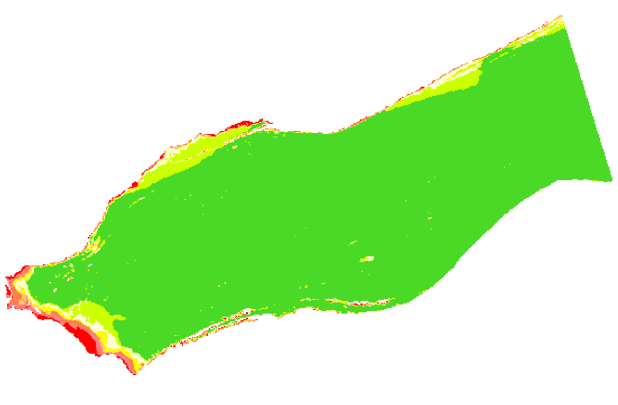
The final output will have values between 1 and 8. A cell value of 1 represents parts of the glacier tongue that disappeared after 2014, a value of 2 represents parts of the glacier tongue that disappeared after 2015, a value of three represents parts of the glacier that disappeared after 2016, and so on. Cells with a maximum value of 8 represent the remaining extent of the glacier.
To better visualize this trend, we can change the symbolization of the output raster.
Right-click on the layer in the layers pane and go to "Set colour table". Then, press the defined tab and locate the "gyr" colour table under the "Name of colour table" drop-down menu. Check the invert box and press run. This resulting layer will look like this:
The second step of the time series detection is to conduct a simple statistical analysis of the rate and magnitude of change in the glacier tongue.
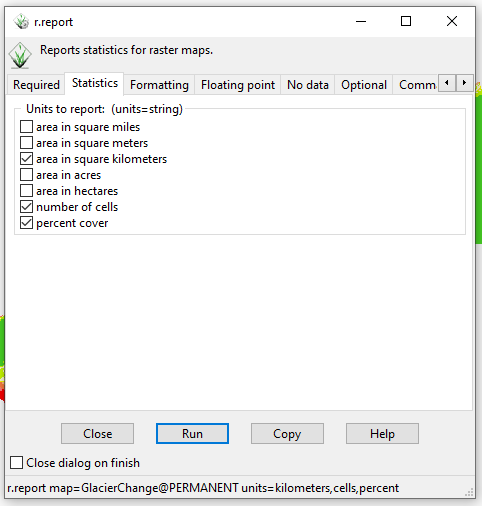
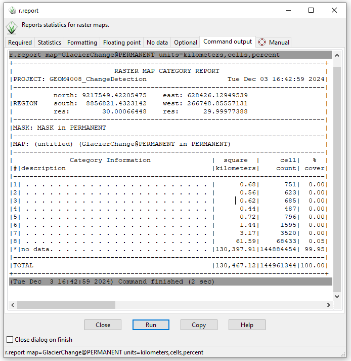
Go to "Raster" > "Reports and statistics" > "Sum area by raster by raster map and category [r.report]". Select the GlacierChange raster, and check the "area in kilometres under the "Statistics" tab—press run.
This tool's output is a statistical report that provides the total area in square kilometres, cell count, and percent cover of each raster class.
The glacier tongue lost 0.68 km2 of ice between 2014 and 2015, 0.56 km2 between 2015 and 2016, 0.62 km2 between 2016 and 2018, 0.44 km2 between 2018 and 2019, 0.72 km2 between 2019 and 2020, 1.44 km2 between 2022 and 2023, and 3.17 km2 between 2023 and 2024. In total, the glacier lost 7.63 km2 or 11% of the glacier tongue area between 2014 and 2024
Conclusion
In conclusion, the tutorial teaches users about the impacts of climate change in the Arctic through an informative demonstration of GRASS GIS and universal raster calculator-based raster analysis. Some key concepts demonstrated in this tutorial were raster math, NDSI, raster masking, raster reclassification, and statistical analysis of rasters.
