Difference between revisions of "Network Analysis: Finding shortest path in QGIS"
Joshgoutte (talk | contribs) (→Introduction: Updated version) |
|||
| (160 intermediate revisions by 3 users not shown) | |||
| Line 1: | Line 1: | ||
==Purpose== |
==Purpose== |
||
This project aims to introduce the various capabilities of open source softwares and their ability to solve spatial problems. The idea of open software was introduced during the GEOM 4008 course at Carleton University, and the finalized work of this course is this tutorial which was originally published in 2014, edited in 2017 and 2021. It will attempt to explain a helpful tool in Quantum GIS (QGIS), an open source software, that can identify the shortest path between two points in a network based on either distance or time. We have to use the Network Analysis tool in the processing toolbar for this tutorial and I will go step-by-step on how we can do that. |
|||
This is a project based on the knowledge taken during the GEOM 4008 course in Carleton University. This tutorial aims to explain for the reader one of the tools used in Quantum GIS for defining shortest path distance. QGIS is an open source software, used widely in previous tutorials of the GEOM 4008 course. Refering to previous tutorials done before on this course you may find more information regarding the QGIS software. Check: [http://http://gracilis.carleton.ca/CUOSGwiki/index.php/Georeferencing_Raster_Imagery_in_QGIS_using_Vector_Data link Georeferencing in QGIS], |
|||
QGIS is widely used in previous tutorials of the GEOM 4008 course. |
|||
== Introduction == |
== Introduction == |
||
Calculating the shortest distance between two points is a |
Calculating the shortest distance between two points is a very common spatial problem that appears in our daily life quite often. In [https://www.arcgis.com/features/ ArcGIS] software (not open source), this problem can be solved using |
||
the Network Analysis tool. We use an identically named tool on QGIS and it is an ideal open source alternative. This tutorial will explore that QGIS tool as a solution for finding the shortest path distance or time by calculating cumulative cost between two points in a network. Installing, activating and configuring the tool in the latest version of QGIS 3.20.3 are the most important steps to start this project. The use of the tool is to measure a cumulative cost based on length between two nodes of a network. Measurements take in consideration either the first case, when the speed limit is the same for all the roads (edges of our network) or the second case, when the speed limit differs for some selected roads. |
|||
== Data == |
== Data == |
||
The data are provided by City of Ottawa Open Data Catalog. |
The data are provided by [http://data.ottawa.ca/ City of Ottawa Open Data Catalog]. In order to create the network, a few files are required. Download the "Roads Centrelines" shapefile, the "Outdoor Rinks" shapefile, the "Water" shapefile and lastly the "Wards 2010" shapefile, in addition of to the "Basketball courts" , "Tennis courts", "Outdoor Wading Pools", "Cycling Network", "O-Train" "O-Train Stage 1" and their corresponding station shapefiles. |
||
The shapefiles should be located in the same folder, within which we are going to store our work. Create a folder in your desired directory called "NetworkAnalysis" or something similar in order to store the downloaded shapefiles as well as any outputs that are generated. |
|||
== Acquiring QGIS (version 2.6) == |
|||
== Acquiring QGIS (version 3.20.3) == |
|||
*You need to install Quantum GIS version 2.6 in order to get activate the road graph plugin.[[File:QgisLOGO.PNG]] |
|||
*You need to install the newest version of Quantum GIS (version 3.20.3 at the time of editing this tutorial) in order to activate the road graph plugin. |
|||
*You may go to this link : [https://www.qgis.org/en/site/forusers/download.html QGIS(v.2.6)] in order to download the QGIS version that is suitable to the operating system you are working on. |
|||
*You may go to this link : [http://www.qgis.org/en/site/forusers/download.html QGIS Download] in order to download the QGIS version that is suitable to the operating system you are working on. |
|||
* After the software is downloaded and ready to execute, we double click the QGIS shortcut icon on Desktop. The GQIS window opens. |
|||
* After the software is downloaded and ready to execute, double click the QGIS shortcut icon on your Desktop or search for it in the Start Menu. The QGIS window opens, and we are ready to begin. |
|||
== Set up the Environment== |
== Set up the Environment== |
||
The type of the data that we are going to work are vector data. The first step is importing the |
The type of the data that we are going to work are vector data. The first step is importing the data into QGIS. |
||
===Add vector data=== |
===Add vector data=== |
||
In Layer menu, select Add layer and choose Add Vector Layer. Another option is click the Add Vector Layer button of the toolbar[[File:Vector.PNG]] |
In Layer menu, select Add layer and choose Add Vector Layer. Another option is click the Add Vector Layer button of the toolbar.[[File:Vector.PNG]]. |
||
Add each of the layers(in .shp format) individually. |
|||
===Projection=== |
===Projection=== |
||
All the layers |
All the layers are to be projected under EPSG:2951 - NAD83(CSRS) / MTM zone 9 projection. Right click on the layer, select Properties, you then go into Source, search and select the appropriate projection. Click apply to see your changes and repeat with your 4 layers. This process can done for all the layers that we are working with, however they should all have the same CRS automatically.[[File:Source2.JPG|200px|thumb|left]]. |
||
[[File:Projection.PNG|200px|thumb|left]] |
|||
| Line 42: | Line 51: | ||
=== Area of |
=== Area of Interest (AOI)=== |
||
The project is focused on determining the shortest path between |
The project is focused on determining the shortest path between the outdoor rink at Brewer Park and one at Jack Purcell Park in downtown Ottawa. By creating an area of interest, or AOI, we can effectively reduce the amount of useless data in the output. In larger data sets, creating an AOI may also reduce processing times. |
||
*In Layer menu, choose Create Layer, then New Shapefile layer and the New Vector Layer window will show up. The AOI should be a polygon. |
*In Layer menu, choose Create Layer, then New Shapefile layer and the New Vector Layer window will show up. The AOI should be a polygon. |
||
*Click the AOI layer. |
*Click the AOI layer. |
||
*Click the Toggle on button to start editing the layer. [[File:Toggle1.PNG]] |
*Click the Toggle on button to start editing the layer. Alternatively, right click on your new layer in the Layers Panel on the left hand side and toggle editing "On" [[File:Toggle1.PNG]] |
||
* |
*Zoom to the scale that meets your needs by holding the CTRL button and using the scroll wheel on your mouse. To create the polygon, find the polygon create tool begin by clicking in each of the four corners of your current zoom extent. This ensures that your AOI has 90 degree angles and crisp lines. On the last point of the polygon, right click to finish creating it. |
||
[[File:AOI2.PNG|200px|thumb|left]] |
[[File:AOI2.PNG|200px|thumb|left]] |
||
| Line 67: | Line 76: | ||
=== Union tool=== |
|||
The data for the trains in Ottawa divided by old O-Train and the new LRT so if we want to be able to find the path with a train, we need to join those two together |
|||
*Go on the vector menu, scroll over Geoprocessing tools and select "Union" |
|||
*You will find page like the one in the figure below where you will select the input and overlay layer which can be "O-Train" and "O-Train Stage 1" |
|||
*Select Run and you should have you Ottawa train network |
|||
[[File:Union20.png|200px|thumb|left]] |
|||
Also the AOI needs to be projected with the same projections as other layers. |
|||
*Right click on AOI layer |
|||
*Select Properties |
|||
*Choose CRS |
|||
*Filter the code 2951 in the filter tab to find faster the projection NAD83 MTM9 |
|||
[[File:Filter.PNG|200px|thumb|left]] |
|||
| Line 104: | Line 111: | ||
===Clip tool=== |
===Clip tool=== |
||
This tool is found under the Geoprocessing Tools of vector data. It is useful to clip the roads shapefile by using as clipping area the AOI. |
|||
Now we will clip all of our layers to match the extent of the AOI. Navigate to the Vector menu at the top of the QGIS user interface, put the cursor on Geoprocessing tools and select Clip. You select "Run as a Batch Process". This allows us to clip all of our desired layers at once using one tool (Please note that the Batch Processing Tool requires at least 3 input layers to function). |
|||
[[File:Clip.png|200px|thumb|left]] |
|||
[[File:Clip20.png|200px|thumb|left]] |
|||
*Input vector is the layer we want to clip: ''Roads'' |
|||
*Clip layer is the ''AOI'' that we just created |
|||
*Output shapefile is specified by us. Refer to the file folder you created to hold all shapefiles and outputs earlier in the tutorial. |
|||
| Line 121: | Line 131: | ||
The same steps were conducted also for the museums shapefile. |
|||
*Input vector is the layer we want to clip: ''Museums'' |
|||
*Clip layer is the ''AOI'' we just created |
|||
*Output shapefile is specified by us. it should be browsed in the same folder where other shapefiles are stored. |
|||
[[File:Clip function.PNG|200px|thumb|left]] |
|||
| Line 140: | Line 145: | ||
=== Symbology=== |
|||
To improve the visual appeal and usability of the map that we create, we should symbolize the different layers to meet our needs instead of staying with the defaults. Firstly, we will symbolize roads based on their type (Street, Boulevard, Parkway, Highway etc.) |
|||
To that on QGIS, you need to do a rule based classification: |
|||
[[File:Rulebased.png|200px|thumb|right]] |
|||
*Right click on the clipped roads layer |
|||
=== Symbology=== |
|||
It would be good to categorize the clipped roads that we got lately. We categorized them by type. |
|||
*Right click on the roads layer |
|||
*Select Properties |
*Select Properties |
||
*Choose '' |
*Choose ''Symbology'' and in the scroll down menu selected "Rule Based" |
||
*You will then set a rule using an expression such as "SUBCLASS" IN ('HIGHWAY', 'FREEWAY') to combine those two classes of roads |
|||
*Double click on the symbols of each roads type to edit them. |
|||
*This is necessary if you have over 10 road types that you cannot sort otherwise. |
|||
*Classify to as many road names as you want |
|||
[[File:Symbology.png|200px|thumb|left]] |
|||
The train data can be symbolized with the rail symbol available on QGIS. |
|||
Any other added features that we added can also be customized so the map: tennis court(green dot), wading pool(blue dot), etc... |
|||
We can also label the clipped rinks file in order to see the names of the rinks. |
|||
*Right click on the clipped rinks layer |
|||
*Select Properties |
|||
*Choose "Labels" and at the top of the Labels window, select "Show labels for this layer", using "PARKNAME" as the label field. |
|||
I do not however recommend doing it for the tennis, basketball and wading pools as they share locations in many cases and it could be a cause for clutter. |
|||
The results should look similar to the screenshot below. |
|||
[[File:OverviewSymb.png|200px|thumb|left]] |
|||
| Line 170: | Line 183: | ||
== Road Graph Plugin== |
|||
The Road Graph Plugin is a C++ plugin for QGIS that calculates the shortest path between two points on any polyline layer and plots this path over the road network. |
|||
Main features: |
|||
* Calculates path, as well as length and travel time. |
|||
* Optimizes by length or by travel time. |
|||
* Exports path to a vector layer. |
|||
* Highlights roads directions (this is slow and used mainly for debug purposes and for the settings testing). |
|||
=== Activate the Tool=== |
|||
[[File:plugin.PNG|400px|thumb|left]] |
|||
---- |
|||
To activate the Road Graph plugin: |
|||
---- |
|||
*Start the Plugin Manager by clicking on the QGIS main window’s menu item ''Plugins'' ‣ ''Manage and Install Plugins''. |
|||
* A dialog window appears. Write ''road'' on the search tab |
|||
*It will automatically appear the ''road graph plugin'' and check it on. (this plugin is already installed in the repository, when we installed the software in our computers ) |
|||
*Go back to your work window |
|||
*This panel will appear in your interface |
|||
[[File:Panel.PNG|200px|thumb|left]] |
|||
*If the plugin doesn't show automatically in your interface, go to ''View ‣ Panels'' and ensure that ''Shortest path'' has a '''check mark''' next to it. |
|||
===Configure the Tool=== |
|||
[[File:Config.PNG|200px|thumb|left]] |
|||
Time Unit and Distance Unit we leave as default in hour and kilometer. Topology tolerance: In case if there is a gap between two lines to treat them as continuous, the topology tolerance may be applied, for example 10m. In our case we left as default 0. On the Transportation Layer, we choose the layer of the roads. In this case the clipped roads. For the direction field we leave as default. In other cases, while in the attribute table we might have a direction field, we might use the value of this field for direction. For this project we don't have any data for the direction. We keep the speed limit as default. And we choose the speed limit value under the Default Settings tab. For this example the speed was chosen 60 km/h as shown in Figure below. |
|||
[[File:Setting.PNG|200px|thumb|left]] |
|||
| Line 293: | Line 202: | ||
== Network Analysis == |
|||
The Network Analysis tool for QGIS calculates the shortest path between two points on any polyline layer and plots this path over the road network. |
|||
Main features: |
|||
- Calculates path, as well as the cost(length or time). |
|||
- Optimizes by length or by travel time. |
|||
- Exports path to a vector layer. |
|||
| Line 301: | Line 216: | ||
===Using the Tool=== |
|||
* Go to the ''Processing'' menu |
|||
* Select the "Toolbar" menu, the processing toolbar should now appear on the right of your workspace |
|||
* Select the ''Network Analysis'' drop down menu, you will then find "Shortest path(point to point)" which you then select |
|||
You should see an image like the one on the figure below |
|||
[[File:NetAnaly.PNG|200px|thumb|left]] |
|||
=== Use the Tool=== |
|||
Suppose we want to calculate the distance in length from Canadian Museum of Nature to Canadian War Museum. |
|||
In the plugin panel, click on the Capture Point button next to the Start field: |
|||
[[File:St.PNG|200px|thumb|left]] |
|||
| Line 319: | Line 236: | ||
*Click point that represent Canadian Museum of Nature as start point. |
|||
*Use the ''Capture Point'' button next to the ''Stop field'' and capture the point of Canadian War Museum. |
|||
[[File:Start.PNG|400px|thumb|left]] |
|||
| Line 330: | Line 244: | ||
To start, you will need to choose a vector layer which will represent the network. This is where you have to choose your mode of transport, if you want to use the bike, choose the cycling network; the train, choose the union train shapefile; and for the cars, pick the roads. |
|||
You will then have the option for the shortest or fastest path, I will give the instructions for both: |
|||
| Line 340: | Line 256: | ||
====Shortest:==== |
|||
*Select the shortest option in the menu |
|||
Suppose you are playing hockey at Brewer Park after class, but your friend wants to meet at Jack Purcell rink downtown. We need to calculate the shortest possible route in length from Brewer Park to Jack Purcell Park |
|||
*For the Start field, click the 3 dots and select a point to start on the map, Brewer Park for our example |
|||
*For the end point, do the same but select Jack Purcell for our example |
|||
*For the direction field, are able to use the FLOW field in the attribute table. |
|||
*Click on the ''Calculate'' button to see the solution: |
|||
*For Forward direction, specify "FT", and use "TF" for backward direction. These abbreviations mean "From - To" and "To - From" respectively, meaning From a specified point to an edge (in this case, a road polyline) and vice-versa for TF. Leave the value for two-way direction blank. This allows the tool to factor one-way roads into its calculations, instead of sending you on an impossible route through the city. |
|||
[[File:Length.PNG|200px|thumb|left]] |
|||
*Choose the speed limit value under the Default Settings tab. For this example the speed was chosen 50 km/h as shown in Figure below. |
|||
* The results should look like the figure on the right |
|||
[[File:SettingsNAShort.png|200px|thumb|left]] |
|||
[[File:ShortestPathMap.png|200px|thumb|right]] |
|||
| Line 369: | Line 293: | ||
The result for the shortest path is shown below. This is a simple case, where the speed mode is the '''same''' for all the streets, 60 km/h. |
|||
[[File:Res1.PNG|400px|thumb|left]] |
|||
| Line 378: | Line 300: | ||
===Setting Speed Criteria=== |
|||
To be able to do the fastest route we need to set the speed criteria |
|||
===Using Criteria=== |
|||
What happens when different streets in the network road have different speed limits? |
What happens when different streets in the network road have different speed limits? |
||
| Line 404: | Line 310: | ||
*Right click on the roads layer. |
*Right click on the roads layer. |
||
*Open attribute table and select the |
*Open attribute table and select the Pencil to set on the edit mode . [[File:Toggle1.PNG]] |
||
*After that click the New Column icon.[[File:NewC.PNG]] |
*After that click the New Column icon.[[File:NewC.PNG]] |
||
| Line 411: | Line 317: | ||
====Queries==== |
====Queries==== |
||
Now we |
Now we run a Field Calculator expression within the road layer that will specify the speed limit 60 km/h for the Streets, 50 for Avenues, 80 for Roads and 40 km/h for the rest of the road types. |
||
Open up the attribute table for the clipped roads file and select the Pencil in the top left corner. Then, open up the Field Calculator.(figure below) |
|||
*On the bottom left corner of the Attribute Table, there is a ''Show All Features'' button. Click on the arrow and select ''Column Filter'' *Then choose for example '''TYPE''', because we want to select the private roads. |
|||
*As you write rt_private automatically will appear the ''Advanced Filter expression''. |
|||
* ''Select private roads and assign the speed limit 50 by using Advanced Filter expression'' |
|||
[[File: |
[[File:FieldCalculatorButton.jpg|200px|thumb|left]] |
||
| Line 432: | Line 336: | ||
From here, we can write a simple expression that will populate the SPEED field created earlier with our desired values. Enter the expression into the Field Calculator as is shown below, or specify your own values for different road types. The speeds defined here are totally arbitrary, and are simply meant to show the functionality of the field calculator to remove the need for individually defining each street's speed limit. |
|||
[[File:FieldCalcul.png|200px|thumb|left]] |
|||
* ''Select public roads with name BRONSON and assign the speed limit 60 by using Advanced Filter expression'' |
|||
[[File:Bronson.PNG|200px|thumb|left]] |
|||
| Line 453: | Line 357: | ||
* ''Select public roads with name GLOUCESTER and assign the speed limit 45 by using Advanced Filter expression'' |
|||
[[File:Gloucester.PNG|200px|thumb|left]] |
|||
After assigning the speed limits for each selection we save the edits by clicking the save button and then click the toggle button again to turn off the edit mode.[[File:Save.PNG]] |
|||
====Fastest:==== |
|||
Go back to the Network Analysis tool like you did earlier |
|||
*Select "Fastest" in the path to calculate |
|||
*Select your start and end point it could be the same two again |
|||
*Enter the same direction information for the shortest path |
|||
*Now under the speed field, select the "SPEED" field |
|||
*You can keep the average speed from earlier and the topographic tolerance as well |
|||
If you run this, you should get the fastest path(results shown on the right) |
|||
[[File:SettingsNAFast.PNG|200px|thumb|left]] |
|||
[[File:FastestPathMap.PNG|200px|thumb|right]] |
|||
| Line 471: | Line 384: | ||
* ''Select the rest of the public roads and assign the speed limit 30 by using Advanced Filter expression'' |
|||
[[File:Not.PNG|200px|thumb|left]] |
|||
| Line 488: | Line 398: | ||
After assigning the speed limits for each selection we save the edits by clicking the save button and then click the toggle button again to turn off the edit mode.[[File:Save.PNG]] |
|||
====Use the tool after criteria is done==== |
|||
*You can switch back and forth between these criteria, recalculating each shortest and fastest paths, and note the changes in cost taken. In this particular example, the only difference between the shortest and fastest route is a single right turn. |
|||
*Check the Vector ‣ Road graph ‣ Road graph settings to ensure that it’s set up as explained previously in this tutorial, but with the ''Speed'' value set to the '''SPEED''' field you just created. |
|||
*In the Shortest path panel, click the Start point button. |
|||
*Set the starting point to where the point of Museum of Nature is located. |
|||
*Set the end point to the Museum of War location. |
|||
*The last operation is to export the output as a shapefile, by clicking the ''Export'' button on the Shortest path panel. |
|||
Let's look at the differences between the paths, the fastest in red and the shortest in black(below) |
|||
*In the Criterion drop-down list in the Shortest path panel, select '''Length'''. |
|||
*'''Click Calculate'''. The route will be calculated for the shortest distance: |
|||
[[File: |
[[File:ComparisonRoad.PNG|200px|thumb|left]] |
||
| Line 524: | Line 429: | ||
Notice the values of ''Length'' and ''Time'' in the ''Shortest Path'' panel. |
|||
| Line 530: | Line 434: | ||
And this is the result graphically of the shortest path in distance |
|||
[[File:SpeedLRes.PNG|400px|thumb|left]] |
|||
*Set the ''Criterion'' to ''Time''. |
|||
*Click Calculate again. The route will be calculated for the shortest time: |
|||
[[File:Time.PNG|200px|thumb|left]] |
|||
*You can switch back and forth between these criteria, recalculating each time, and note the changes in the ''Length'' and ''Time'' taken. |
|||
The Shortest Time path result as shown below |
|||
[[File:TimeRes.PNG|400px|thumb|left]] |
|||
*The last operation is to export the output as a shapefile, by clicking the ''Export'' button on the Shortest path panel. |
|||
== Conclusion == |
== Conclusion == |
||
The Network Analysis tool for QGIS is a useful utility for solving any cost-distance query that one might have. The tool itself is very user-friendly and intuitive and can really help in finding the best route using whichever criteria designated. One could verify that they set up the tool properly by checking if the outputs for the the fastest and shortest path are the same, indicating that the SPEED field wasn't created properly. This tool is slightly limited in the sense that if we would like to calculate the distance between two points in miles or the speed field is in miles/hour, the tool will not give us solution, because by default it supports only kilometers and meters. One way to solve this would be to convert miles to meters or km through another field calculator expression. |
|||
Road graph plugin used in QGIS, helped defining the shortest and the fastest way to get from Canadian Museum of Nature to Canadian Museum of War, based on the cost length. It is important to verify the settings. You could verify from the output that if the speed limit is the same in all the roads, the shortest distance would be the same route for the length and time cost. While if we apply different speed limits for different segments of roads, than there is difference between the shortest path way for length cost, compare to shortest path way for time cost. |
|||
==Future work== |
==Future work== |
||
This solution could be further improved when we can combine modes of transport, for example, wanting to bike to the train. It can also be improved if we can find a way to incorporate traffic using some indices and the inclusion of real time data would really benefit such a model, however maybe more in a web map than QGIS. Having the data to update construction sites, road closures and other separated incidents that would affect the model would be great but mostly the responsibility of the data supplier. Also for the delivery companies such as UPS, Canada Post could calculate the most cost effective road which a software like this would permit, the possibility to add multiple points would also be pretty good. |
|||
Future work might be creating Drive Time isochrones in QGIS. Site analyses can benefit greatly from using “drive-time” isochrones to define the study area. In ArcGIS this is called Sercive Area. It might be helpful ([http://http://pgrouting.org/ pgRouting]) open source software to create the nodes network, which each of them would define a start and an end point for different segments that create the network. This is benefical for airports. If the location of airports are consider to be the nodes of the network, then a routable network graph with adequate weights would be created by pgRouting. |
|||
The first step is to find the closest network node to every airport. The next one is to calculate drive times between network nodes and “airport nodes”. The resulting point layer than can be imported into QGIS. Using TIN interpolation (from Interpolation plugin), we can calculate a continuous cost surface. And Contour function (from GDALTools) yields drive time isochrones. Based on this analysis, it is possible to determine how many inhabitants live within one hour driving distance from an airport or how many people have to drive longer than e.g. ninety minutes to reach any airport. |
|||
== References == |
== References == |
||
*7.3. lesson: Network Analysis¶. QGIS Documentation. (2020, June 5). Retrieved September 30, 2021, from https://docs.qgis.org/3.4/en/docs/training_manual/vector_analysis/network_analysis.html. |
|||
* |
*ArcGIS. (2014) Service Area Analysis. Retrieved Dec 15, 2014 http://help.arcgis.com/en/arcgisdesktop/10.0/help/index.html#//004700000048000000 |
||
*QGIS. (2021) Download QGIS for your Platform. Retrieved on September 30, 2021 from http://www.qgis.org/en/site/forusers/download.html |
|||
* |
*City of Ottawa Open Data Catalog (2013).Roadways Retrieved on December. 15, 2014 http://data.ottawa.ca/dataset/roadways |
||
* |
*City of Ottawa Open Data CatalogMuseums (2013). Museums Retrieved on December. 15, 2014 http://data.ottawa.ca/dataset/museums |
||
*QGIS. (2014) Download QGIS for your Platform. Retrieved on December 15, 2014 from http://www.qgis.org/en/site/forusers/download.html |
|||
*QGIS. Blog (2014) Retrieved on December 16, 2014 http://planet.qgis.org/planet/tag/drive%20time%20isochrones/ |
|||
*Roadways (2013). City of Ottawa Open Data Catalog Retrieved on December 15, 2014 http://data.ottawa.ca/dataset/roadways |
|||
Latest revision as of 14:06, 30 September 2021
Contents
Purpose
This project aims to introduce the various capabilities of open source softwares and their ability to solve spatial problems. The idea of open software was introduced during the GEOM 4008 course at Carleton University, and the finalized work of this course is this tutorial which was originally published in 2014, edited in 2017 and 2021. It will attempt to explain a helpful tool in Quantum GIS (QGIS), an open source software, that can identify the shortest path between two points in a network based on either distance or time. We have to use the Network Analysis tool in the processing toolbar for this tutorial and I will go step-by-step on how we can do that. QGIS is widely used in previous tutorials of the GEOM 4008 course.
Introduction
Calculating the shortest distance between two points is a very common spatial problem that appears in our daily life quite often. In ArcGIS software (not open source), this problem can be solved using the Network Analysis tool. We use an identically named tool on QGIS and it is an ideal open source alternative. This tutorial will explore that QGIS tool as a solution for finding the shortest path distance or time by calculating cumulative cost between two points in a network. Installing, activating and configuring the tool in the latest version of QGIS 3.20.3 are the most important steps to start this project. The use of the tool is to measure a cumulative cost based on length between two nodes of a network. Measurements take in consideration either the first case, when the speed limit is the same for all the roads (edges of our network) or the second case, when the speed limit differs for some selected roads.
Data
The data are provided by City of Ottawa Open Data Catalog. In order to create the network, a few files are required. Download the "Roads Centrelines" shapefile, the "Outdoor Rinks" shapefile, the "Water" shapefile and lastly the "Wards 2010" shapefile, in addition of to the "Basketball courts" , "Tennis courts", "Outdoor Wading Pools", "Cycling Network", "O-Train" "O-Train Stage 1" and their corresponding station shapefiles.
The shapefiles should be located in the same folder, within which we are going to store our work. Create a folder in your desired directory called "NetworkAnalysis" or something similar in order to store the downloaded shapefiles as well as any outputs that are generated.
Acquiring QGIS (version 3.20.3)
- You need to install the newest version of Quantum GIS (version 3.20.3 at the time of editing this tutorial) in order to activate the road graph plugin.
- You may go to this link : QGIS Download in order to download the QGIS version that is suitable to the operating system you are working on.
- After the software is downloaded and ready to execute, double click the QGIS shortcut icon on your Desktop or search for it in the Start Menu. The QGIS window opens, and we are ready to begin.
Set up the Environment
The type of the data that we are going to work are vector data. The first step is importing the data into QGIS.
Add vector data
In Layer menu, select Add layer and choose Add Vector Layer. Another option is click the Add Vector Layer button of the toolbar..
Add each of the layers(in .shp format) individually.
Projection
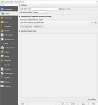
All the layers are to be projected under EPSG:2951 - NAD83(CSRS) / MTM zone 9 projection. Right click on the layer, select Properties, you then go into Source, search and select the appropriate projection. Click apply to see your changes and repeat with your 4 layers. This process can done for all the layers that we are working with, however they should all have the same CRS automatically.
.
Area of Interest (AOI)
The project is focused on determining the shortest path between the outdoor rink at Brewer Park and one at Jack Purcell Park in downtown Ottawa. By creating an area of interest, or AOI, we can effectively reduce the amount of useless data in the output. In larger data sets, creating an AOI may also reduce processing times.
- In Layer menu, choose Create Layer, then New Shapefile layer and the New Vector Layer window will show up. The AOI should be a polygon.
- Click the AOI layer.
- Click the Toggle on button to start editing the layer. Alternatively, right click on your new layer in the Layers Panel on the left hand side and toggle editing "On"
- Zoom to the scale that meets your needs by holding the CTRL button and using the scroll wheel on your mouse. To create the polygon, find the polygon create tool begin by clicking in each of the four corners of your current zoom extent. This ensures that your AOI has 90 degree angles and crisp lines. On the last point of the polygon, right click to finish creating it.
Union tool
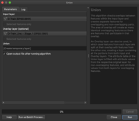
The data for the trains in Ottawa divided by old O-Train and the new LRT so if we want to be able to find the path with a train, we need to join those two together
- Go on the vector menu, scroll over Geoprocessing tools and select "Union"
- You will find page like the one in the figure below where you will select the input and overlay layer which can be "O-Train" and "O-Train Stage 1"
- Select Run and you should have you Ottawa train network
Clip tool
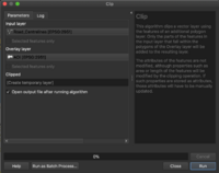
Now we will clip all of our layers to match the extent of the AOI. Navigate to the Vector menu at the top of the QGIS user interface, put the cursor on Geoprocessing tools and select Clip. You select "Run as a Batch Process". This allows us to clip all of our desired layers at once using one tool (Please note that the Batch Processing Tool requires at least 3 input layers to function).
- Input vector is the layer we want to clip: Roads
- Clip layer is the AOI that we just created
- Output shapefile is specified by us. Refer to the file folder you created to hold all shapefiles and outputs earlier in the tutorial.
Symbology
To improve the visual appeal and usability of the map that we create, we should symbolize the different layers to meet our needs instead of staying with the defaults. Firstly, we will symbolize roads based on their type (Street, Boulevard, Parkway, Highway etc.)
To that on QGIS, you need to do a rule based classification:
- Right click on the clipped roads layer
- Select Properties
- Choose Symbology and in the scroll down menu selected "Rule Based"
- You will then set a rule using an expression such as "SUBCLASS" IN ('HIGHWAY', 'FREEWAY') to combine those two classes of roads
- This is necessary if you have over 10 road types that you cannot sort otherwise.
- Classify to as many road names as you want
The train data can be symbolized with the rail symbol available on QGIS.
Any other added features that we added can also be customized so the map: tennis court(green dot), wading pool(blue dot), etc...
We can also label the clipped rinks file in order to see the names of the rinks.
- Right click on the clipped rinks layer
- Select Properties
- Choose "Labels" and at the top of the Labels window, select "Show labels for this layer", using "PARKNAME" as the label field.
I do not however recommend doing it for the tennis, basketball and wading pools as they share locations in many cases and it could be a cause for clutter.
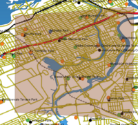
The results should look similar to the screenshot below.
Network Analysis
The Network Analysis tool for QGIS calculates the shortest path between two points on any polyline layer and plots this path over the road network.
Main features:
   - Calculates path, as well as the cost(length or time).
   - Optimizes by length or by travel time.
   - Exports path to a vector layer.
Using the Tool
- Go to the Processing menu
- Select the "Toolbar" menu, the processing toolbar should now appear on the right of your workspace
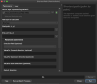
- Select the Network Analysis drop down menu, you will then find "Shortest path(point to point)" which you then select
You should see an image like the one on the figure below
To start, you will need to choose a vector layer which will represent the network. This is where you have to choose your mode of transport, if you want to use the bike, choose the cycling network; the train, choose the union train shapefile; and for the cars, pick the roads.
You will then have the option for the shortest or fastest path, I will give the instructions for both:
Shortest:
- Select the shortest option in the menu
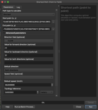
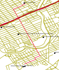
Suppose you are playing hockey at Brewer Park after class, but your friend wants to meet at Jack Purcell rink downtown. We need to calculate the shortest possible route in length from Brewer Park to Jack Purcell Park
- For the Start field, click the 3 dots and select a point to start on the map, Brewer Park for our example
- For the end point, do the same but select Jack Purcell for our example
- For the direction field, are able to use the FLOW field in the attribute table.
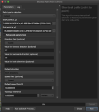
- For Forward direction, specify "FT", and use "TF" for backward direction. These abbreviations mean "From - To" and "To - From" respectively, meaning From a specified point to an edge (in this case, a road polyline) and vice-versa for TF. Leave the value for two-way direction blank. This allows the tool to factor one-way roads into its calculations, instead of sending you on an impossible route through the city.
- Choose the speed limit value under the Default Settings tab. For this example the speed was chosen 50 km/h as shown in Figure below.
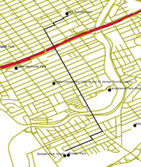
- The results should look like the figure on the right
Setting Speed Criteria
To be able to do the fastest route we need to set the speed criteria What happens when different streets in the network road have different speed limits?
The idea is to set different speed limits for some of the selected streets by us. In this case we had to add a new field in the roads layer and call it Speed.
Create New Field
- Right click on the roads layer.
- Call this new column SPEED, and give it the type Whole number (integer) with a width of 3.
Queries
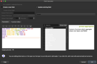
Now we run a Field Calculator expression within the road layer that will specify the speed limit 60 km/h for the Streets, 50 for Avenues, 80 for Roads and 40 km/h for the rest of the road types.
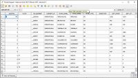
Open up the attribute table for the clipped roads file and select the Pencil in the top left corner. Then, open up the Field Calculator.(figure below)
From here, we can write a simple expression that will populate the SPEED field created earlier with our desired values. Enter the expression into the Field Calculator as is shown below, or specify your own values for different road types. The speeds defined here are totally arbitrary, and are simply meant to show the functionality of the field calculator to remove the need for individually defining each street's speed limit.
After assigning the speed limits for each selection we save the edits by clicking the save button and then click the toggle button again to turn off the edit mode.
Fastest:
Go back to the Network Analysis tool like you did earlier
- Select "Fastest" in the path to calculate
- Select your start and end point it could be the same two again
- Enter the same direction information for the shortest path
- Now under the speed field, select the "SPEED" field
- You can keep the average speed from earlier and the topographic tolerance as well
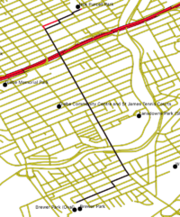
If you run this, you should get the fastest path(results shown on the right)
- You can switch back and forth between these criteria, recalculating each shortest and fastest paths, and note the changes in cost taken. In this particular example, the only difference between the shortest and fastest route is a single right turn.
- The last operation is to export the output as a shapefile, by clicking the Export button on the Shortest path panel.
Let's look at the differences between the paths, the fastest in red and the shortest in black(below)
Conclusion
The Network Analysis tool for QGIS is a useful utility for solving any cost-distance query that one might have. The tool itself is very user-friendly and intuitive and can really help in finding the best route using whichever criteria designated. One could verify that they set up the tool properly by checking if the outputs for the the fastest and shortest path are the same, indicating that the SPEED field wasn't created properly. This tool is slightly limited in the sense that if we would like to calculate the distance between two points in miles or the speed field is in miles/hour, the tool will not give us solution, because by default it supports only kilometers and meters. One way to solve this would be to convert miles to meters or km through another field calculator expression.
Future work
This solution could be further improved when we can combine modes of transport, for example, wanting to bike to the train. It can also be improved if we can find a way to incorporate traffic using some indices and the inclusion of real time data would really benefit such a model, however maybe more in a web map than QGIS. Having the data to update construction sites, road closures and other separated incidents that would affect the model would be great but mostly the responsibility of the data supplier. Also for the delivery companies such as UPS, Canada Post could calculate the most cost effective road which a software like this would permit, the possibility to add multiple points would also be pretty good.
References
- 7.3. lesson: Network Analysis¶. QGIS Documentation. (2020, June 5). Retrieved September 30, 2021, from https://docs.qgis.org/3.4/en/docs/training_manual/vector_analysis/network_analysis.html.
- ArcGIS. (2014) Service Area Analysis. Retrieved Dec 15, 2014 http://help.arcgis.com/en/arcgisdesktop/10.0/help/index.html#//004700000048000000
- QGIS. (2021) Download QGIS for your Platform. Retrieved on September 30, 2021 from http://www.qgis.org/en/site/forusers/download.html
- City of Ottawa Open Data Catalog (2013).Roadways Retrieved on December. 15, 2014 http://data.ottawa.ca/dataset/roadways
- City of Ottawa Open Data CatalogMuseums (2013). Museums Retrieved on December. 15, 2014 http://data.ottawa.ca/dataset/museums
