Highly Effective Construction of Thematic Maps

OpenJUMP Tutorial by Thomas Brown - Revised by Didier Soeharjono

Introduction

About OpenJUMP

OpenJUMP is a Free and Open Source Software for Geospatial (FOSS4G) that is similar to other popular Geographic Information Systems (GIS) such as ArcGIS or QGIS. Originally founded by Vivid Solutions in 2002, this software was formerly known as JUMP (Java Unified Mapping Platform) before being discontinued in 2006. Since then, it has been renamed as OpenJUMP in recognition to the original Canadian development team, but also due to the fact that further contribution is open to the public. Nowadays, maintenance efforts are accomplished through The JUMP Pilot Program (JPP), an association committed to coordinating its development. The JPP consists of various separate organizations and global volunteer developers.

Languages

• Tamil
• French
• Czech
• Finnish
• Italian 
• English
• Portuguese
• Telugu
• Malay
• Brazilian
• Portuguese
• Chinese (Simplified)
• German
• Japanese
• Spanish
• Hungarian

Intended Audience

• Non-Profit Organizations
• Government
• Science/Research
• Developers
• End Users/Desktop
• Agriculture

User Interface

• Java Swing

Programming Language

• Java

Capabilities

• Cross-platform compatibility with Windows, Linux, Unix, MacOSX (with Java installed)
• Read & write the following vector file formats: CSV, DXF, GeoJSON, GML, JML, OSM, SHP and more
• Read & write the following raster file formats: ASC, BMP, DCX, ECW, GeoTIFF, GIF, JPEG, PNG, TIFF and more
• Read recognized data formats from compressed files (zip, tar, tar.gz, tar.bz and more)
• Database access: read ArcSDE, MySQL, Oracle, PostGIS, SpatialLite & write PostGIS
  • Note: Compatibility with certain file formats may require an additional plugin
• BeanShell & Python consoles allows to script
• Tools include: Queries, Analysis, Statistics, Generate, Warp, QA, Measure & more
• Availability of various third-party extension plugins
• Allows to store, edit, process, analyze & display spatial data

Why use OpenJUMP?

The feature that really sets it apart from other programs is that the main focus of its tools and functionality leans more towards style through the ease of editing geometry and attribute data. Additionally, its friendly layout results with a rapid learning curve.

Purpose

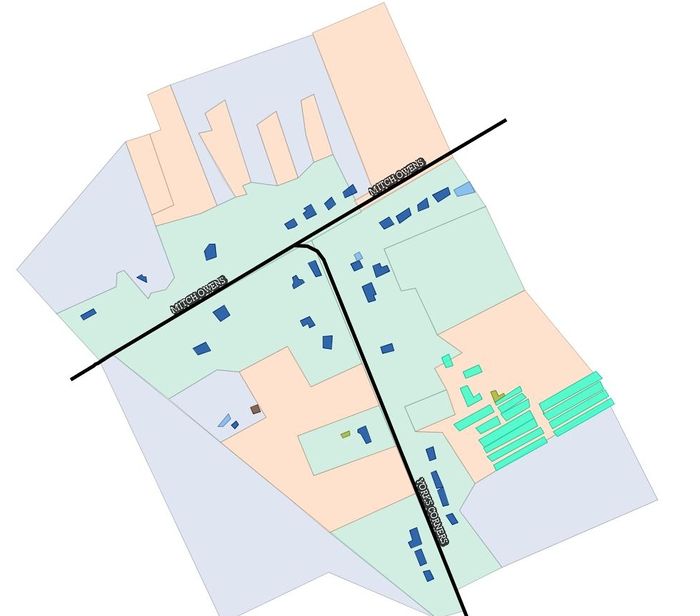
This tutorial will demonstrate the construction of a common thematic map displaying the land use throughout Ottawa in OpenJUMP (such as the one shown in Figure 1.1). In contrast to reference maps which focuses on physical features, a thematic map has the main goal of displaying a particular theme in an area. These maps can be seen as an infographic that communicates information to the viewer. As seen in this exercise, their production in GIS software requires stacking multiple data layers together and then modifying the map’s appearance in order to enhance the visualization of the thematic data. Throughout this process, the user will determine various potentials linked to this software through editing the attributes and symbology of the provided data. Furthermore, it will help become more familiar with this user-friendly open source GIS.

Figure 1.1 shows a thematic map built and styled in OpenJUMP

The Process

Obtaining OpenJUMP and data

Step 1: Downloading OpenJUMP
OpenJUMP can be downloaded through the following link [1] by clicking the green ‘Download’ button.

Step 2: Downloading the data
The Ottawa Thematic Data can be downloaded through the following link [2] by clicking the red 'Land Use 2010 - Direct Download' link.
Note: Since this data is from a licensed dataset, it is only available to Carleton students, staff and faculty.

Starting OpenJUMP and importing data

Step 3: Starting OpenJUMP
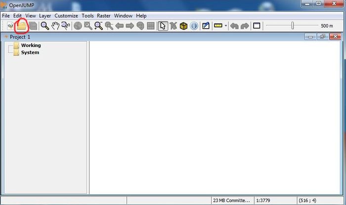
OpenJUMP starts up by clicking the icon, the main screen shown in Figure 1.2 should appear shortly after.

Step 4: Importing the data
Adding files is done by using the folder icon circled in red as seen in Figure 1.2. In this case, we will be importing the 'LandUse_2010.shp' file which can be found where the previously downloaded data was saved. Right now would be a good time to save your project by clicking on the 'File' tab and then the 'Save Project As' button.
Note: it is important to save your project frequently to avoid losing any progress.

Figure 1.2 shows the starting interface of OpenJUMP and highlights the icon for importing files.

Manipulating the data

Step 5: Extracting the data
The 'LandUse_2010' data will appear as one single layer even though it consists of mulitple attributes. This results with the image being displayed in one single color, even though our goal is to portray each land use type by different colors. To achieve this, click on the 'Edit' tab, then scroll over 'Extract' before choosing the 'Extract Layer by attribute' button. In the pop-up window, select 'LU_2010' as the attribute. This will result with the creation of a new folder named 'Extract' in the content pane which shows each attribute as a single layer.

Step 6: Reclassifying land use layers
By referring to the 'LandUse_2010_Legend.xlsx' Microsoft Excel file that comes in the downloaded data folder, we can classify the land use layers into 9 different types. Each layers will be reclassified into the following categories:

• Residential:R1; R2; R3; R3-3; R4-x; R-4; R-5
• Commercial:C1; C2; C3; OF
• Industrial:M1; M2
• Institutional:I1; I2; I3; I3-r; I4; I5
• Recreational:RE-A; RE-A-s; RE-p; RE-p-s
• Utilities:TR; UT; COMM; ST
• Water:Water; IW
• Landcover:OS; AG; FT; QS; ROS; WL; WL-FT
• Other:V1; V2

To do so in OpenJUMP, we can select the appropriate layers for each category then right-click and choose the 'Combine selected layers' button. This will combine all the selected layers into one single layer, we will then rename the new 'Combined' layer to the appropriate category name by double-clicking on the label. This process will have to repeated until the 9 reclassified categories have been created and renamed.

Imported Files

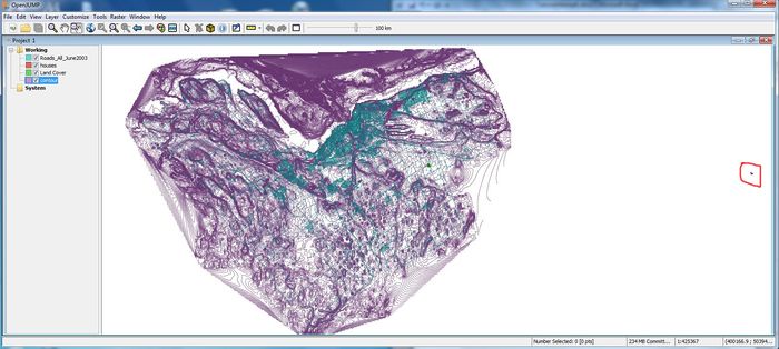
Once the files are imported into OpenJUMP they will be given a default color and style scheme. If one layer is visually blocking another it just needs to be selected in the table of contents in the upper left of Figure 1.3 and dragged to below the layer that it is blocking. A common problem with OpenJUMP is that input files with different projections can end up far apart on the map as shown in Figure 1.3 where the shapefile of houses (circled in red) ended up far to the right.

Figure 1.3 shows how shapefiles look when loaded into OpenJUMP. The shapefiles shown represent contours and roads for the Ottawa area as well as some digitized land use and house polygons for a small area hereby called Smallville.

Manipulating Files with Tools

Since OpenJUMP is designed for easily changing the way that maps look, putting a shapefile back in the right place is fairly simple:

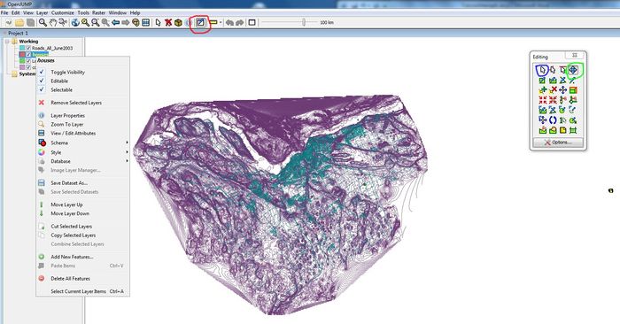
• First, right click the shapefile that you want to adjust in the table of contents and make sure that “Toggle Visibility”, “Editable” and “Selectable” are all checked (as shown in Figure 1.4).

• Second, open the “Editing Toolbox” which is the icon circled in red on Figure 1.4 and select the “Select Features Tool” (the icon circled in blue in Figure 1.4) and use it to select the shape that you are editing.

• Third, select the “Move Selected Items” tool (the icon circled in green on Figure 1.4) and use your mouse to drag the shape to wherever it should be.

Figure 1.4 shows the “Editing Toolbox” being used to move the houses shapefile back to where it belongs.

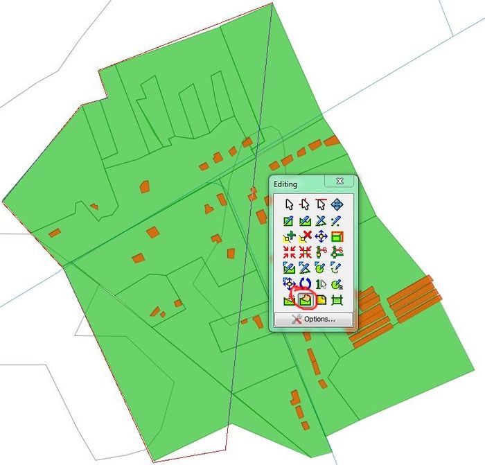
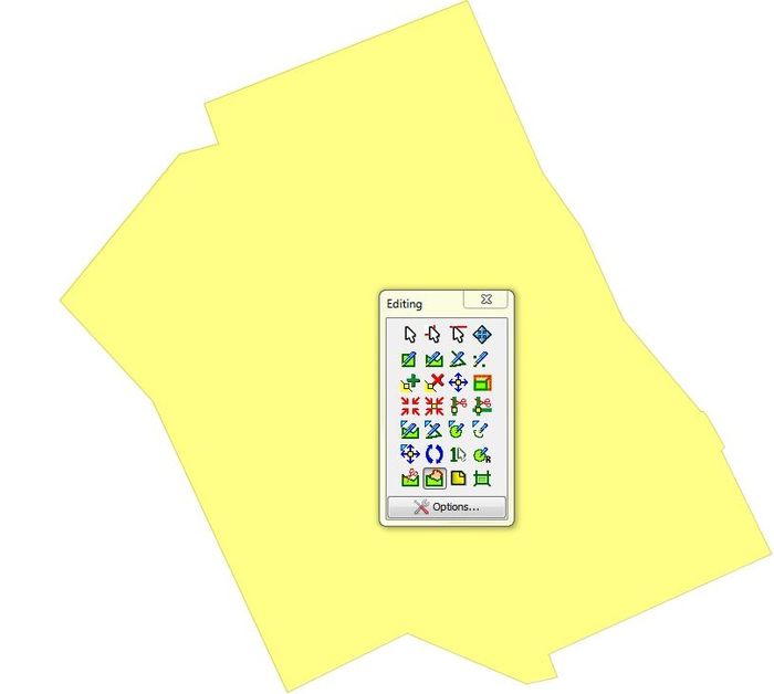
For many maps it will be necessary to clip input files so that they are all within the study area. The first step for this is to design an area of interest mask polygon. The polygon is built using the “Auto Complete Polygon” tool (the icon in the toolbar circled in red in Figure 1.5). A user can then select vertices of the polygon (as shown in Figure 1.5) and double click to let the polygon finish as shown in Figure 1.6.Note: If a layer is still "Selectable" when right clicked on, the polygon will be joined with it.

Figures 1.5 (left) and 1.6 (right) show the “Auto Complete Polygon” being used and the resulting AOI polygon respectively.

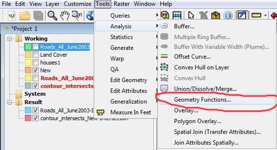
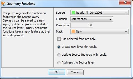
Using one polygon to cut another requires the “Geometry Functions” tool highlighted in red in Figure 1.7. This tool changes the geometry of a shapefile based on the function field. In the case of the example the “Source” layer is where the roads layer is used, the “Funtion” is “Intersection” to find out where the roads and mask intersect spatially and the “Mask” field is where the Area of Interest (AOI) polygon can be added. It is not necessary to change the defaults on the other input fields. The tool and the input are shown in Figure 1.8. Once roads are clipped, any other lines can do through the same process (in the example this includes contours).

Figure 1.7 shows how to navigate to the Geometry Functions Tool Figure 1.8 shows the inputs used for the Geometry Functions tool

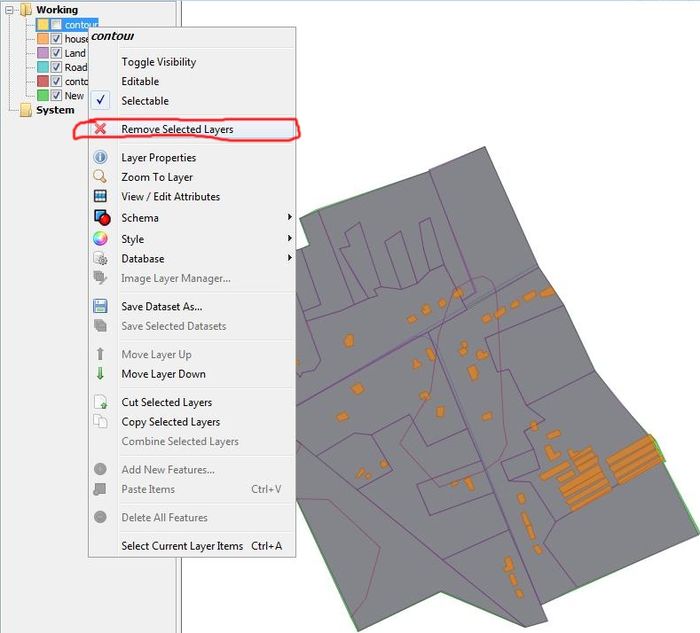
With the new layers formed the original layers can be removed by right clicking on them and selecting “Remove Selected Layers” as shown with the output of the tool in Figure 1.9.

Figure 1.9 shows the output from the Geometry Functions tool and how to remove layers.

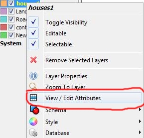
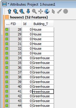
At this point all of the shape files are in place and it is a good opportunity to edit attributes. Do this by right clicking the layer in table of contents and selecting “View / Edit Layer Attributes” (as shown in Figure 1.10). In the case of the example “Greenhouse” is spelt incorrectly in the attribute table. By making the layer editable and entering the attribute table all attributes are manually editable.

Figures 1.10 (left) and 1.11 (right) show how to navigate to the “View / Edit Attributes” function and how editing an attribute table looks respectively. Styles and Symbology

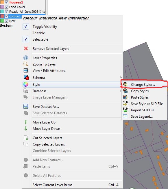
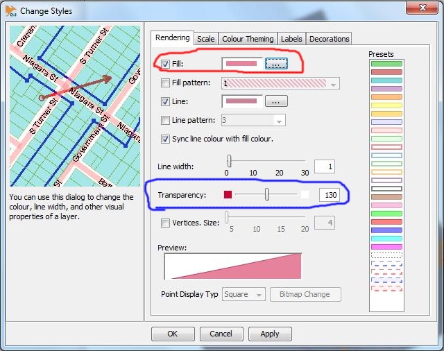
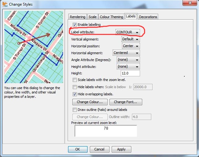
With the files all manipulated correctly it is now time to use OpenJUMP’s stylizing functionality. The first shapefiles to be modified are the lines (contours and roads). Right click the contours file in the table of contents and navigate to “Change Style” ( circled in red in Figure 2.1). From the Change Stlyes interface there are many options. In the case of contour lines on a map they commonly are a light, semi-transparent colour. Note how this is reflected in 2.2 by selecting a light pink colour as the fill (circled in red) and setting the transparency to 130 out of 255 (circled in blue). In Figure 2.3 the “Labels” tab has been opened. It is common for maps with contour lines to label them based on the elevation they represent. Note that the “Label Attribute” (circled in red) has been set to “CONTOUR” (elevation value) and everything else is left as a default. Feel free to mess around with labelling styles but for now the elevation just appearing besides the contour line looks nice.

Figure 2.1 shows how to navigate to Change Styles in OpenJUMP Figure 2.2 shows the rendering preferences for contours Figure 2.3 shows the Labels preferences for contours

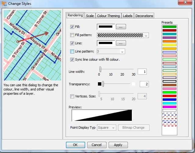
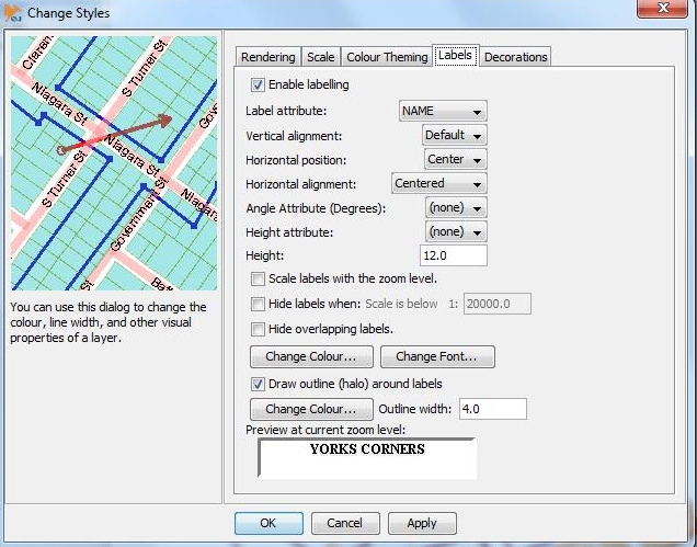
Since roads are also in the form of lines the steps to stylize them are the same. In the case of the example they are given a black fill with no transparency (configuration shown in Figure 2.4). The labels for the street names have been changed to bold Times New Roman font with a halo outline that makes features, that would normally make the names more difficult to read, slightly transparent (configuration shown in Figure 2.5).

Figures 2.4 (left) and 2.5 (right) show, respectively, the rendering and labelling configuration for roads.

The polygon shapefiles (land use and houses) will implement colour theming to make them easier to interpret visually. Figure 2.6 shows how this is done through the “Colour Theming” tab. The “Attribute” drop-down menu can be used to select the field that will be used to separate the different colours in the map. The “Colour Scheme” drop-down menu contains many options for which colour the layer will be represented by. The table that is influenced by these changes can also be edited manually. In Figure 2.6 the colours being used have all been added manually. The colours used for both land use and houses are all personal preference and are done the same way.

Figure 2.6 shows the colour theming configuration for land use Figure 2.7 shows the colour theming configuration for houses

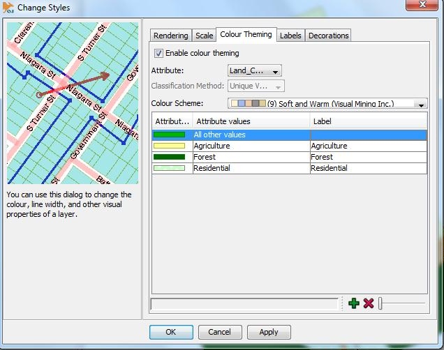
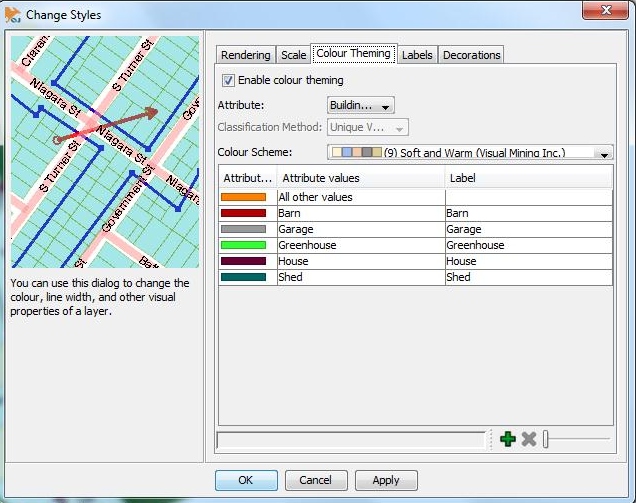
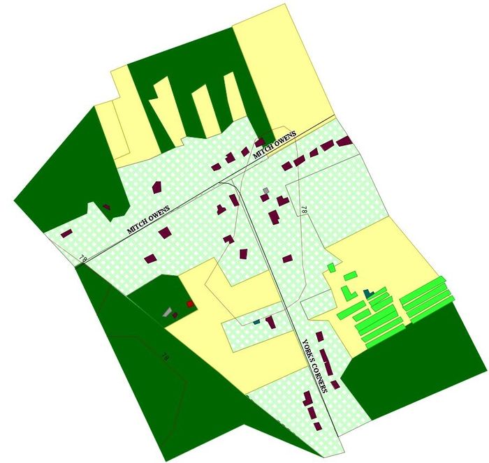
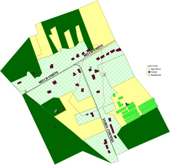
Once the colour theming is complete the output will be a final map product like Figure 2.8. This final map product makes it easy to interpret what is on the map in addition to being visually appealing.

Figure 2.8 shows the final map project developed in the example.

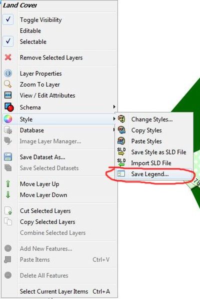
At this point adding a legend will help with interpreting the map. Right click the layer that would benefit from a legend (in the case of this project it will be for land use). Select Styles -> Save Legend (as shown in Figure 2.9). Save the legend somewhere memorable and then use the Add Files icon from Figure 1.2 to load in the Legend image. The image may end up far away from the map itself so use the method shown in Figure 1.4 to move it to the desired location. Once in place the end result should look like Figure 2.10 below.

Figure 2.9 shows how to save a legend for a layer Figure 2.10 shows the final map product with a legend.

Styled Layer Descriptor

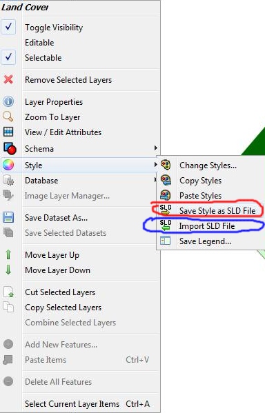
Since shapefiles in general will not store visual styles as soon as the mapping program is closed and reopened all of that work styling is wasted. Styled Layer Descriptors (SLD) retain style information for layer and can be built, imported and exported using OpenJUMP. These files are not only useful for maintaining style in OpenJUMP but since they are written in Extensible Markup Language (XML) they are universally useful for styling webmaps. To build an SLD simply right click on the layer in the table of contents and select Style->Save Style as SLD File (red circle in Figure 3.1). From there the SLD file is stored and can be imported for a layer at any point using the Style->Import SLD File option from the same menu (blue circle in Figure 3.1).

Figure 3.1 shows how to navigate to the SLD uses.

Conclusion

You now have a final map product and SLD files for styling. Try different styles as OpenJUMP has a really great variety.

Thanks for Reading my Tutorial

Kangaroo GIF