Difference between revisions of "Intro to GRASS workshop"
| Line 1: | Line 1: | ||
= Introduction to GRASS GIS (7.6.1) = |
= Introduction to GRASS GIS (7.6.1) = |
||
This document was written based on an older version that originally accompanied |
This document was written based on an older version that originally accompanied a workshop given at Carleton University on 17 October 2011, in the Department of Geography and Environmental Studies' main GIS lab (Loeb A200). Anyone is welcome to adapt it for other purposes or to help improve and keep this tutorial up to date (see CC license conditions at the bottom left of the page). |
||
The expected audience for this tutorial consists of people that are new to GRASS GIS, but not new to GIS in general - i.e. we do not explain basic GIS concepts, and when the software "behaves" very similarly to other common GIS software, this tutorial does not provide much in the way of detailed instructions (e.g. choosing map symbology). |
The expected audience for this tutorial consists of people that are new to GRASS GIS, but not new to GIS in general - i.e. we do not explain basic GIS concepts, and when the software "behaves" very similarly to other common GIS software, this tutorial does not provide much in the way of detailed instructions (e.g. choosing map symbology). |
||
Latest revision as of 19:56, 28 October 2019
Contents
- 1 Introduction to GRASS GIS (7.6.1)
- 1.1 Getting Started
- 1.2 Importing Vector Data
- 1.3 Controlling the map display
- 1.4 Importing raster data
- 1.5 Analysis example: classification
- 1.6 Analysis example: map algebra to calculate NDVI
- 1.7 Analysis example: vector query, and extracting raster values at vector locations
- 1.8 Analysis example: interpolation (and importing ASCII point data)
- 1.9 Other resources
Introduction to GRASS GIS (7.6.1)
This document was written based on an older version that originally accompanied a workshop given at Carleton University on 17 October 2011, in the Department of Geography and Environmental Studies' main GIS lab (Loeb A200). Anyone is welcome to adapt it for other purposes or to help improve and keep this tutorial up to date (see CC license conditions at the bottom left of the page).
The expected audience for this tutorial consists of people that are new to GRASS GIS, but not new to GIS in general - i.e. we do not explain basic GIS concepts, and when the software "behaves" very similarly to other common GIS software, this tutorial does not provide much in the way of detailed instructions (e.g. choosing map symbology).
In the following sections, text in bold indicates specific practical steps you should perform on your computer to follow along, whereas the rest of the text offers extra explanation or pointers to other resources.
Getting Started
If GRASS is not already installed on a machine for you, getting the software is probably your first step. In this document, the computing environment will use a 64 bit MS Windows 10 OS. The installation part of the tutorial will explain the method for installing pre-compiled binaries.
To download the GRASS GIS software: Go to this detailed software download page, OR visit specific links below.
- Download binaries: WinGRASS 7.6.1 snapshot full installer or LinuxGRASS 7.6.1 snapshot installer or 7.6.1 installer
- Download source code (optional): Download source code packages or Download source code from GitHub repository
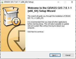
Once the download is completed, run the .exe file to start the installation wizard.
The wizard will guide you to go through the steps in the setup process like any other software setup. Choosing an appropriate location and wait until the installation is completed. Upon completion, click Finish to close the wizard.
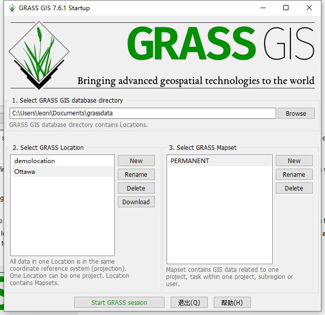
As the default, a shortcut to the GRASS GIS will appear on your desktop. You can also find it under your start menu. Launch GRASS by double-click the shortcut on your desktop. ![]() This will launch a shell script terminal and a graphical interface to choose your GRASS database, location, and maps. These concepts tend to confuse new users, but once you understand the logic used here, file maintenance is taken care of for you to a large degree.
This will launch a shell script terminal and a graphical interface to choose your GRASS database, location, and maps. These concepts tend to confuse new users, but once you understand the logic used here, file maintenance is taken care of for you to a large degree.
The GRASS project has a good introduction to this opening screen on its website, so to avoid reinventing the wheel, please click on this link to bring up the relevant web page. You should be able to piece together the material by reading the full web page online.
Let’s begin with getting your data into a GRASS database, making a fresh database location from scratch. In your GRASS startup window, confirm that the GIS Database Directory is set to an appropriate location such as “C:\Users\YourUserName\Documents\grassdata”, then click on the New button between the Location and Mapset windows. This will open a new window to allow the user to define a new Location.
In the Define new GRASS Location window, give your project an appropriate name in the Project Location. You should avoid spaces in this name, but you can create a more friendly version in the Title. The Location Title is not mandatory, choose a name for it if you like. Click Next.
For the first steps of this tutorial, we are using data distributed by the City of Ottawa, under a license that allows free redistribution and use under the Terms of Use linked here. These files are already retrieved and made easily available for you in the lab, but if you are performing this tutorial on your own, an archive of the data we are using is available here:
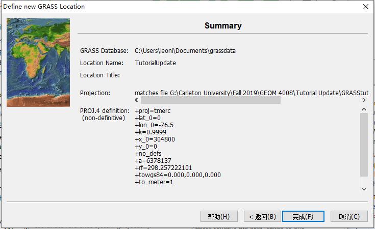
In the next window, choose "Read projection and datum terms from a georeferenced data file". Then use the Browse button no navigate to the georeferenced file (in our case, Roadways.shp), and click Next. In this way, GRASS GIS reads the spatial projection and datum info from your chosen file and displays the projection in the summary window. If there is no error, click Finish.
In the resulting screen, a default extent has been taken from the maximum extents of the roadways data. The resolution parameters do not apply to vector data, however, therefore they are filled with nonsense values.
GRASS uses the concept of a "Window" on your data to define the spatial extent and, for raster processing, the spatial resolution at which all processing is done. This window can be changed at any time, and any data layer can have a different spatial extent and resolution. The Window defines how input layers will be sampled (rasters are resampled at the current window's resolution when data layers have different resolutions). We have just set the default Window for this dataset, which provides an easy way to reset to starting conditions while we're doing GIS processing.
Now you'll be back at the initial GRASS welcome screen, and the new Ottawa location should show up and be selected in the left-most column, with the PERMANENT mapset selected under Accessible mapsets. All locations have at least one mapset, called PERMANENT. Other mapsets can be created to separate out maps belonging to different sub-projects, or to separate maps being created by multiple users sharing the same database. For now, we'll stick with the PERMANENT mapset.
Click the Start GRASS button. The terminal window that was already launched behind the welcome screen will display some introductory text and a GRASS shell prompt (for interactive command-line use), and the GRASS GUI will launch (on these and most modern installations of GRASS, this means the wxPython-based mapping interface).
Importing Vector Data
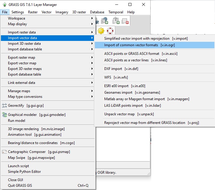
At this point, we have created an empty database - although you pointed at a shapefile to define its spatial attributes, there aren't any data loaded yet. We will import some shapefile from the City of Ottawa GIS data using the OGR-based vector import tool, v.in.ogr, which is accessed in the GUI by selecting the File menu in the GRASS GIS Layer Manager window, then choosing Import vector data | Import of common vector formats.
Previously, if you choose to add the roadway.shp into your PERMANENT mapset, then it is already there but not showing yet. So we don't need to add it again.
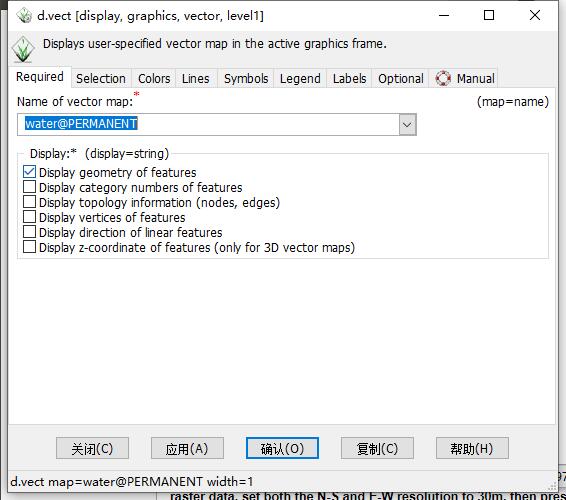
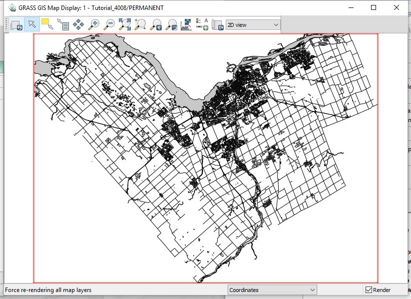
In the resulting window, in the Source name section, click on the Browse button, navigate to where your shapefiles are stored, in our case, let's use the water shapefile as an example, i.e. the water.shp, and press Run. You might notice that after the importing code finishes running, the imported shapefile will not automatically show up as a layer just like your roadway layer. To make it visible, use the add vector map layers tool (The one in the first row of the buttons, or Ctrl+Shift+V). Select your layer in the name of the vector map drop-down menu and press OK. In this way, your shapefiles will show up in the layers window.
Note: To zoom to the layer, simply click on the layer you want to zoom into, and press this ![]() zoom to selected layers button.
zoom to selected layers button.
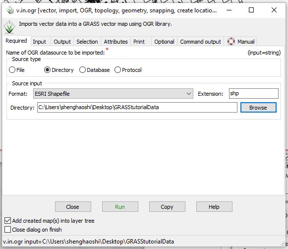
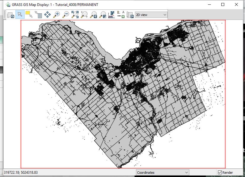
Now we'll import some other vector data layer, but this time we'll use a different approach. Bring up the Import vector data tool again (File|Import vector data|Common import formats), but this time under Source type, choose Directory. Now in the next section, choose the correct format (the ESRI Shapefile) and navigate to the DIRECTORY where your files are stored (select the parent directory, then press Open). When you return to the Import vector data window, all of the OGR-readable data that are found in that directory should show up. Click the Run button.This might take a few minutes.
Note: if you run into an error for file name must start with a letter instead of a number, go to your data folder and rename your file slightly.
The data in those shapefiles are now all stored (separately) in the GRASS database, in GRASS's native data format. The attribute data is, by default, stored in a DBF-format file, just as is used with shapefiles. GRASS can optionally connect to external database servers to hold attribute data, and (with compatible databases) spatial data as well.
Controlling the map display
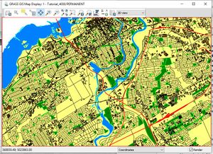
As you'll see in your map window, GRASS does not have very exciting default colors when you add layers to your map - everything is black and white or grey.
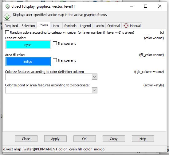
You can adjust the symbology in the GRASS GIS Layer Manager by choosing the Map Layers window tab at the bottom of the window, selecting the layer you want to adjust with your mouse, and either right-clicking on the layer, or clicking on the grey button at right edge of the layer listing, and choosing Properties. In the resulting dialogue box, use the Colors, Lines, Symbols and Labels tabs as necessary to get the kind of symbology you think is appropriate for each layer. Also, just like ArcGIS, you can click and drag the layers to rearrange which layer stays on top and which layer stays at the bottom.
Some interesting characteristics of the map layer properties include the ability to limit the display of objects using SQL queries, and the ability to drive symbology using attribute columns for things like symbol sizes and color schemes. Unfortunately, the City data we're using doesn't have that much in the way of interesting attributes to get very fancy in our map today.
Back in the Layer Manager window, note that right-clicking on the layer while it is selected also lets one:
- set opacity levels for each layer,
- zoom the map to the extent of the selected layer,
- change the current GRASS computational region (the "window" discussed above) to match the currently selected layer,
- remove or rename the layer,
- turn on the editing mode, * rebuild topology for they layer, or
- bring up the attribute data in a new window.
Importing raster data
Now we'll import some raster data, calling on the power of GDAL software to translate from a wide variety of raster formats.
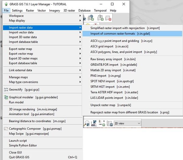
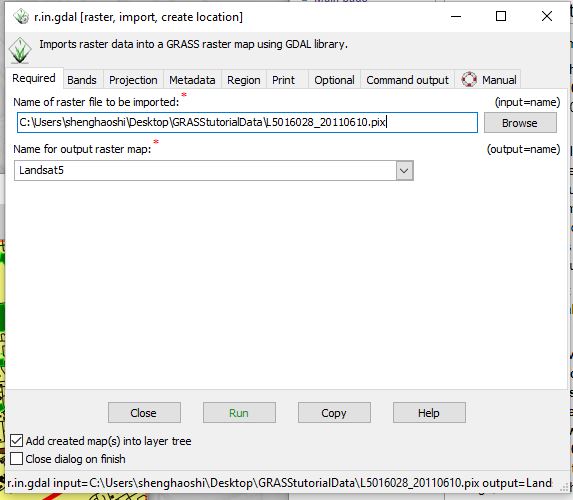
In the File menu, choose Import raster data, then Import of common raster formats. In the resulting window, browse to the file L5016028_20110610.pix, and give the raster map a name such as Landsat5. This is a LANDSAT 5 TM scene, from path 16 row 28, taken on 10 June 2011. It includes most of the City of Ottawa, plus a large region to the north.
Note that in order to speed things up, I have done some preprocessing of the scene, and cropped it somewhat. As discussed in the introductory material about GRASS databases, all files in a given location in the GRASS database must share a common projection and coordinate system. The city data we've used so far and the Landsat image I've downloaded from the USGS archive both are in UTM coordinates, but the datum differs between the two. To fix this, I had to create a separate GRASS location to hold the satellite data at first, then I imported it from GeoTIFF using the same file import tools we've just used above, then I switched back to this GRASS location, and used r.proj (Raster|Develop raster map|Reproject raster map in the menus) to reproject the image files from the other location to this one, specifying a 30m resolution for the reprojection. I then exported all of the bands out to a single PCI .pix format file to speed up our import process.
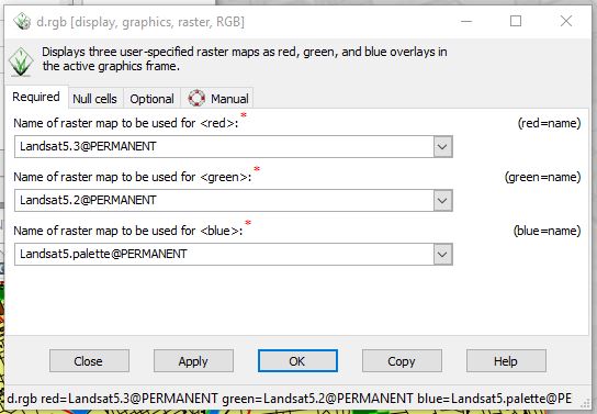
Click on the "Add various raster map layers" button ![]() on the Layer Manager toolbar. Choose the Add RGB map layer option. Fill in the red, green and blue layers by clicking on the downward-facing triangle button to the right of each field, and choosing the following layers for red, green and blue respectively: XXX.3, XXX.2, and XXX.palette. The XXX will be the name you gave it when importing.
on the Layer Manager toolbar. Choose the Add RGB map layer option. Fill in the red, green and blue layers by clicking on the downward-facing triangle button to the right of each field, and choosing the following layers for red, green and blue respectively: XXX.3, XXX.2, and XXX.palette. The XXX will be the name you gave it when importing.
(I'm not sure why band one gets labelled .pallette instead of .1, but it does appear to be the blue band, so for now I'm ignoring this).
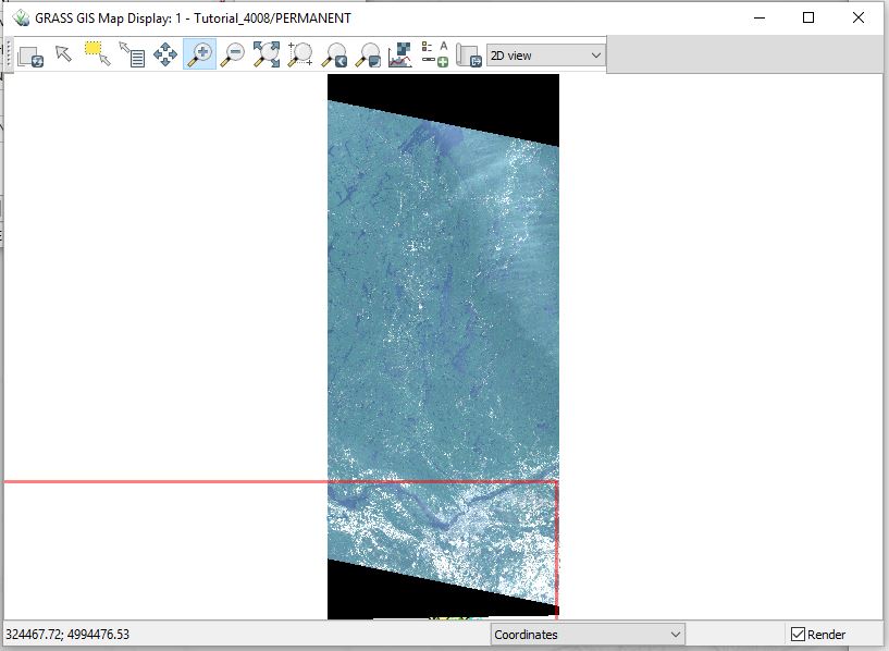
Click OK, and a visible composite should appear in your map window. Feel free to zoom out and explore the image, or examine the other bands.
Analysis example: classification
To demonstrate image processing capabilities of GRASS, we'll quickly perform an unsupervised classification of this image. We'll first do cluster detection on a subset of the bands, then use maximum likelihood classification to assign each pixel a land cover class based on the detected spectral clusters.
Perform the following steps:
- in the Map layers pane of the GRASS GIS Layer Manager window, right click on the satellite image layer, and choose Set computational region from the selected map(s) (this sets the GRASS computational window on the full scene)
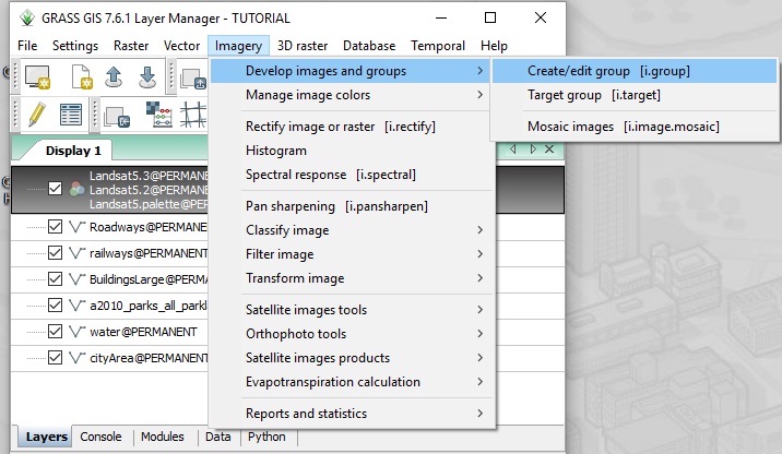
- Under the Imagery menu, choose Develop images and groups|Create/edit group
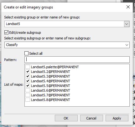
- Check the Edit/create subgroup checkbox, we are creating a new subgroup since we don't have one yet. Fill in "Classify" as the name of the imagery sub-group.
- Click multiple times on the downward-facing triangle to the right of the "Name of raster map(s) to include in group" to choose, in turn each of the layers that end in .palette, .2, .3, .4, and .5 (we are adding the visible and near-infrared bands to a "sub-group" to be analyzed for classification)
- Click the Apply button, then, when it has finished running, Click OK to close the window.
- Under the Imagery menu, choose Classify image|Clustering input for unsupervised classification
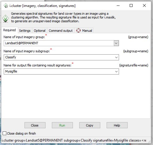
- Choose Landsat5 as the imagery group, Classify as the sub-group, enter Mysigfile as the output signature file.
- In the settings tab,use an initial number of classes of 5
- Click Run, and once it successfully completes the task, click on Close
You have now completed the cluster analysis, and we're ready to classify the image using the detected clusters:
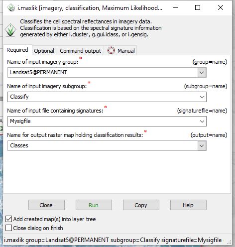
- Under the Imagery menu, choose Classify image|Maximum likelihood classification (MLC)
- For the imagery group, choose Landsat5@PERMANENT, for the name of input imagery subgroup choose Classify, the Name of input file containing signatures is Mysigfile, and enter a name such as "Classes" for the raster map to hold the classification results. Run the module and close the window when it's finished.
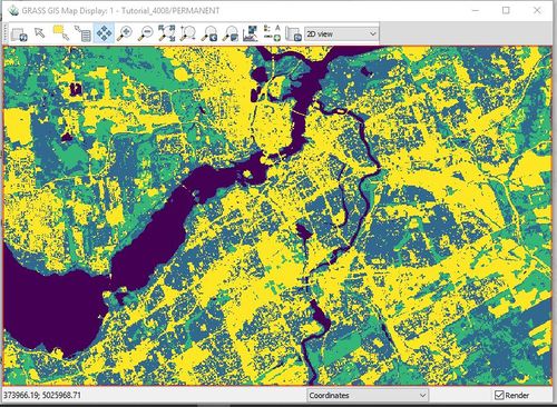
Examine the resulting map, and see what you think of the classification results. To be fair, we haven't exactly conducted a careful training procedure, and the image I downloaded has a fair bit of haze across the whole image, but at this number of classes, it should have done a decent job of picking out at least a water class and some vegetation classes.
Analysis example: map algebra to calculate NDVI
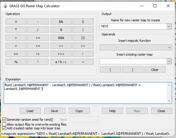
NDVI (normalized difference vegetation index) calculation is a common task with Landsat (or other) imagery. To obtain a proper NDVI map, we would probably want to first apply an atmospheric correction (and obtain an image that didn't have so much haze), but in order to simplify the tutorial and just demonstrating software capabilities, let's ignore rigour and proceed. The map calculator module in GRASS is an interface for the very powerful r.mapcalc program, which makes it easy to build a wide variety of computational models based on raster input layers. We'll use it here to input the formula for NDVI: NDVI = (NIR - Red) / (NIR + Red), where NIR is reflectance in the near infrared (Landsat TM band 4), and Red is red reflectance (Landsat TM band 3).
- From the Raster menu in the Layer Manager, choose Raster map calculator/Raster map calculator
- In the resulting window enter NDVI as the name of the new raster to create, then use the other buttons to create a formula of the form: float( Landsat5.4@PERMANENT - Landsat5.3@PERMANENT ) / float( Landsat5.4@PERMANENT + Landsat5.3@PERMANENT ) (if you use the dropdown menu to insert the layer names, it will add "@PERMANENT" to indicate that these maps are in the PERMANENT mapset - that's fine, but is not needed so you can left them out for simplicity)
In the formula above, the float() function was used to force r.mapcalc to evaluate the addition and subtraction operations using floating-point numbers; since all the input layers were integer maps, it would have otherwise defaulted to using integers for the output map, which leads to a pretty boring 3 category map because NDVI typically varies between 0-1 (with some exceptions).
- Press the Run button to execute the formula
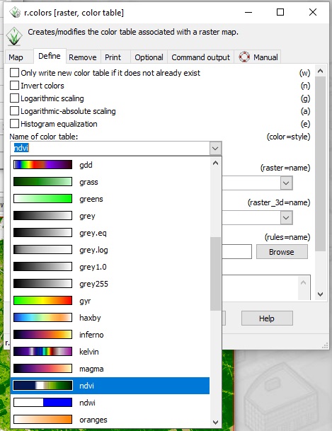
You will get an output of NDVI as a result. However, by just looking at the map display, it is not making a clear sense of where should you expect vegetation coverage. Let's fix that by right click on the NDVI layer in the layer manager, and choose Set color table. In the new window, go to Define tab and choose ndvi as your name of the color table. Press Run.
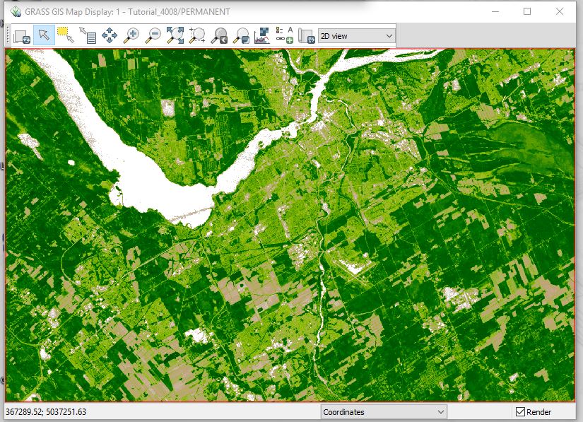
As a result, you will have your map display showing something similar to this: which tells us the vegetation density visually.
- White color represents water body
- Light brown color represents bare lands with little vegetation
- Darker green color represents denser vegetation coverage
- Lighter green color represents sparser vegetation coverage
Analysis example: vector query, and extracting raster values at vector locations
Now let's see what we can learn about the NDVI in Ottawa's parks. To run this analysis on the whole parks data file, however, takes too long for the purposes of tonight's workshop, so first, we'll also subset the parks layer. Do the following steps:
- In the layer manager window, choose Vector|Feature selection|Select by attributes
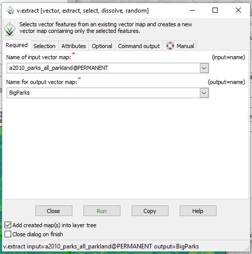
- On the Required tab, for the Name of the input vector map, choose the park shapefile you imported (in my case it is a2010_parks_all_parkland@PERMANENT), and in the Name for output file give the output file a name such as BigParks
- Switch to the Selection tab, and clear all of the geometry type checkboxes except for area, then down in the WHERE condition of SQL statement without 'where' keyword field enter AREA_HA > 15 (this will query the existing map for all areas that have an attribute > 15 in the AREA_HA field)
Note: you can also try the SQL builder by clicking this button
- Click Run, and then when it finishes, click Close.
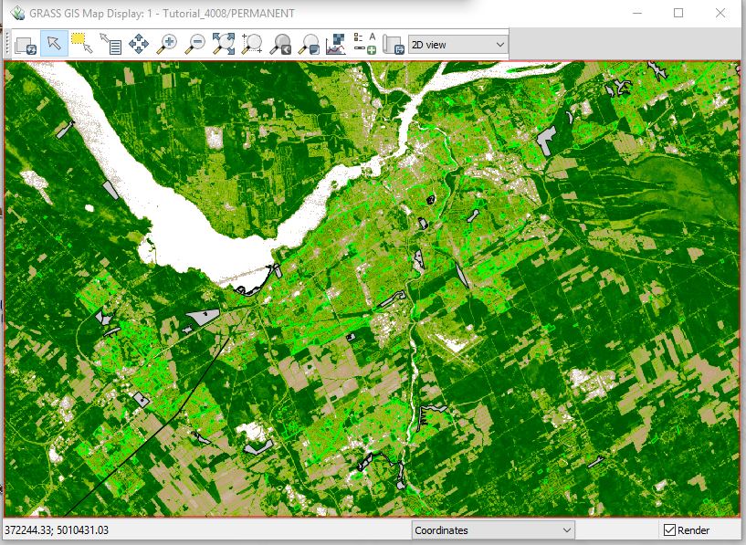
Now in the Map Display window, you can see all the big parks stand out with the default black and grey coloration.
- In the layer manager, on the Map layers pane, select the park layer, right-click on it, and choose to set the computational region to the extent of this file (to avoid wasting time processing the entire region of the NDVI layer)
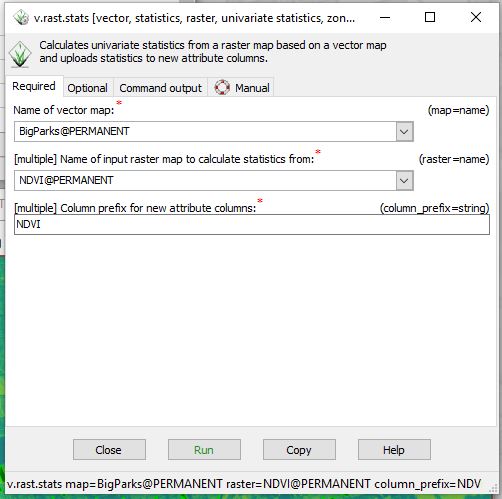
- From the Vector menu, choose Update attributes | Update area attributes from raster In the resulting window, enter BigParks@PERMANENT as the Name of the vector map, NDVI as the name of input raster map, and NDVI as the column prefix. Click Run (it may take a while to process - about 50 seconds on my test machine)
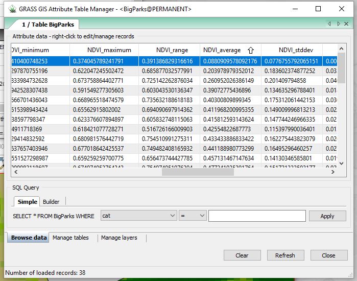
- In the Map layers pane of the Layer Manager, select the BigParks layer, right click on it, and choose Show attribute data
If you scroll to the right in the attribute table, you will see several new fields have been added, describing the distribution of NDVI values that were found in each of the parks.
By click on the title "NDVI_average" we can check the average NDVI value smallest value first. We can tell that most of the big parks have high NDVI value (>0.4) which means dense vegetation coverage, which meets our exception. However, we also find a few big parks with low NDVI value. So let's explore the reason behind it.
We want to check which parks have low NDVI value. To do so, double click on the row, this will highlight the row you chose. Use your mouse to drag and zoom to the park to visually check for the reason. We will show two examples here.
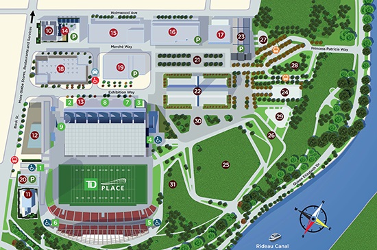
First, by checking the name of the park with the lowest NDVI value (0.088) we know it is the Lansdowne Park Complex, which we know is more of a commercial and recreational center than a typical park with high vegetation coverage.
Map of Lansdowne Park Complex. Source: City of Ottawa
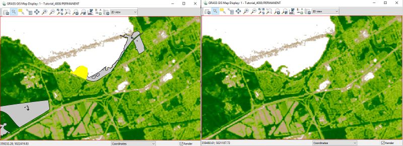
Then, let's look at the big park with the second low NDVI value - the Dick Bell Park. Below is an image of its relative location and the NDVI map of the region. We can tell the reason for low NDVI is likely due to the large water body in the park.
Analysis example: interpolation (and importing ASCII point data)
Now for a classic geography example: house prices! I've searched the locations of a bunch of recent real estate ads in central Ottawa, and placed them into prices.txt - file is included in the zip file you already downloaded to your machine, You can also click here to get the data, and save the file into your data directory.
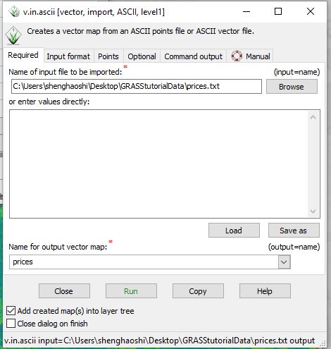
Import the prices data into your GRASS database using File>Import vector data>ASCII points or GRASS ASCII format(v.in.ascii)
- Use browse button to navigate to the prices.txt file, use 'prices' as the Name for output vector map.
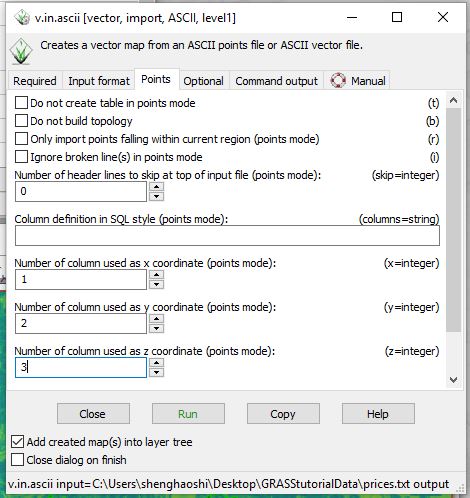
- In the Points tab, specify that the Number of columns used as z coordinate is 3. Hit Run.
Interpolation is actually a fairly complicated topic, and we're not digging too deep into it here, but I'll plough ahead and give you a "teaser" look at the possibilities. We're going to try two different approaches, and you'll see that neither of them does very well at producing a cost surface of housing data with the input I've provided.
- Change the computational region to match that of the prices layer, and then for even better performance, manually zoom into the core of the data in the center of the city, and then use the Zoom Options button on the mapping window to set the computational region to match the display.
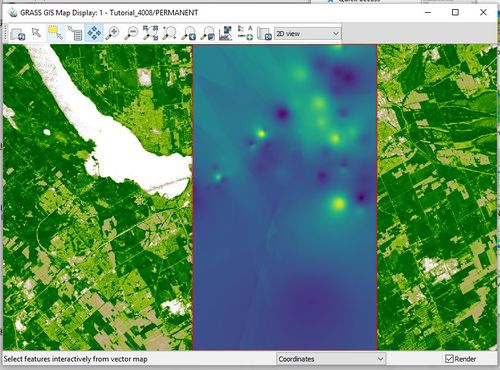
- In the Layer Manager, choose Raster>Interpolate surfaces> Bilinear and bicubic from vector points(v.surf.bspline).
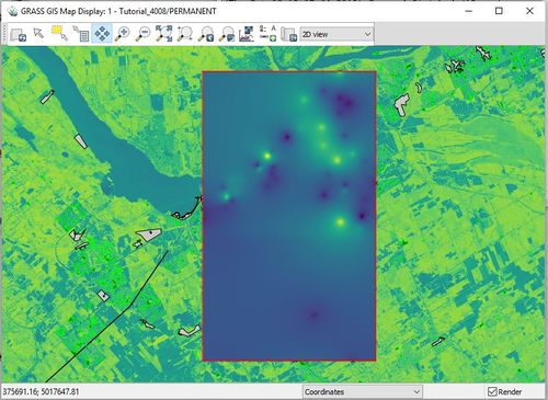
- In the v.surf.bspline window, under Required, chose the prices map. Under the Settings tab, set the layer number to 0. Under the Outputs tab, set the Name of output raster map to priceSurface. Run the module (it will take some time).
The result should look similar to this:
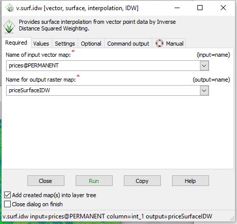
- Now let's try something else, an IDW interpolation. From the Raster menu, choose Interpolate surfaces|IDW from vector points(v.surf.idw). Use prices@PERMANENT as the input, priceSurfaceIDW as the Name for output raster map, and then under the Values tab, specify int_1 as the attribute table column with values to interpolate. Run the module and inspect the output.
Notice any difference between two outputs? That is because Inverse distance weighted (IDW) interpolation makes the assumption that spatial features that are closer to each other are more likely to be related than those that are farther apart. In IDW interpolation, any estimated value is measured base on its surrounding values. The nearer value to your prediction location have the greater impact on how the value is estimated.
I think you'll find that clearly we need more data to make a sensible map of housing prices, but this exercise at least introduced you to interpolations in GRASS. There are many more algorithms available, and the GEOM4008 class will be exploring this in detail in their next assignment.
Other resources
Important resources for more help on GRASS include:
- Open Source GIS: A GRASS GIS Approach, by Neteler and Mitasova (hardcover book, there are 3 editions, all of which have some advantages; available in the Carleton library)
- Main GRASS web site at OSGEO
- GRASS tutorials page
