Difference between revisions of "Network Analysis in Python"
| Line 313: | Line 313: | ||
[[File:10_route_distance.png|500px]] |
[[File:10_route_distance.png|500px]] |
||
===Extracting Street Names=== |
===OPTIONAL: Extracting Street Names=== |
||
Now let's examine the roads taken by this route. The route_to_gdf() tool creates a geodataframe of only the edges traversed by this route. Because it is possible that the same road name appears multiple times, the aggregation must be done slightly differently than simply taking the unique names. |
Now let's examine the roads taken by this route. The route_to_gdf() tool creates a geodataframe of only the edges traversed by this route. Because it is possible that the same road name appears multiple times, the aggregation must be done slightly differently than simply taking the unique names. |
||
| Line 446: | Line 446: | ||
nodes[nodes['highway'].isna()].explore() |
nodes[nodes['highway'].isna()].explore() |
||
</syntaxhighlight> |
</syntaxhighlight> |
||
<pre> |
<pre> |
||
68.74125874125873 |
68.74125874125873 |
||
</pre> |
</pre> |
||
[[File:19_explore_nodes_missing_tags.png|500px]] |
[[File:19_explore_nodes_missing_tags.png|500px]] |
||
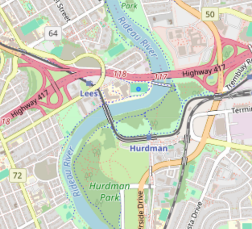
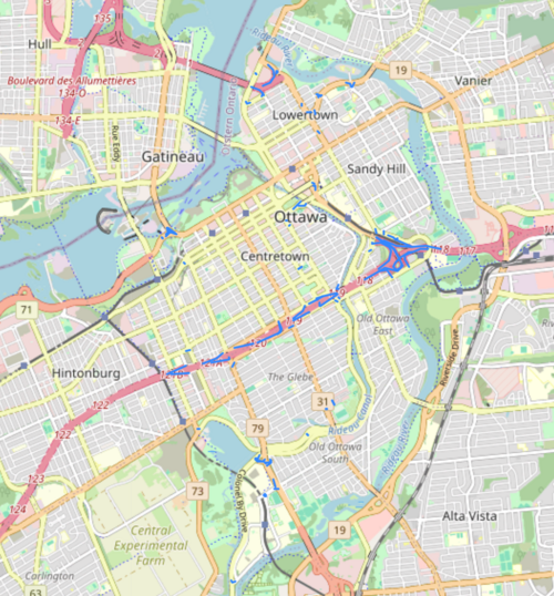
Almost 70% of the nodes in this area are missing a tag. Similar to the edge speeds, some areas are much more complete than others. While there was an easy way to fill in the missing edge speeds, there isn't a simple way to fix this issue, so unfortunately we will have to leave out intersection impedances from our time-weighted shortest path for Ottawa. |
|||
===Time-Based Shortest Path=== |
===Time-Based Shortest Path=== |
||
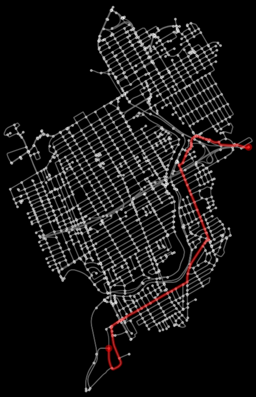
Let's try calculating the shortest path again, this time using travel time as the weight. |
|||
<syntaxhighlight lang="python> |
|||
# Calculate a simple shortest path -> uses Dijkstra's Algorithm |
|||
route2 = osmnx.shortest_path(graph, start_node, end_node, weight='travel_time') |
|||
# Plot the shortest path |
|||
fig, ax = osmnx.plot_graph_route(graph, route2, **pgr_args) |
|||
</syntaxhighlight> |
|||
[[File:20_route_time.png|500px]] |
|||
===OPTIONAL: Extracting Street Names=== |
|||
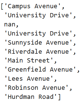
The second route takes a different path. Let's explore the road names again, but this time we can ignore any missing names, which we determined to only be slip lanes, driveways, and highway ramps. |
|||
<syntaxhighlight lang="python> |
|||
# export road names from route |
|||
route_gdf = osmnx.routing.route_to_gdf(graph, route2) # extract this route's edges (road segments) from the larger network |
|||
road_names = list(route_gdf.reset_index()['name']) |
|||
# Because the same road name may appear multiple times, the aggregation must be done slightly differently than simply finding the unique names. |
|||
roads = [] |
|||
for road_name in road_names: |
|||
if pd.isna(road_name): # ignore edges without road names -> highway ramps and slip lanes |
|||
continue |
|||
if not roads or roads[-1] != road_name: |
|||
roads.append(road_name) |
|||
display(roads) |
|||
</syntaxhighlight> |
|||
[[File:21_route_time_streets.png|500px]] |
|||
==Route Comparison== |
==Route Comparison== |
||
Revision as of 06:15, 18 December 2025
Contents
Introduction
Summary
This tutorial explores some basic network analysis in Python using the OSMnx and NetworkX packages.
First, a road network for Ottawa, Ontario is imported from OpenStreetMap (OSM) with OSMnx. The Nominatim API is used for geocoding - no external data download required. Then, shortest path examples are shown, first distance-based, then based on travel time. The incomplete nature of OSM datasets is explored in this section. Additional features such as creating *n* number of shortest paths, comparing routes, plotting with OSMnx, and exporting a route to a shapefile are shown. Finally, a basic example of the Travelling Salesman Problem (TSP) is demonstrated.
This tutorial expects that the reader has at least a basic knowledge of Python.
Setup
Instructions for setting up a Jupyter Notebook with Anaconda and Google Colab are shown below. The only differences between the methods are found when installing the packages, exporting data, and the fact that geocoding seems to take somewhat longer with Google Colab.
Anaconda
A Jupyter Notebook of this tutorial is planned to be provided in the future.
Download Anaconda here
Setup your Conda environment with the required packages by entering the following commands into Anaconda Prompt:
Create an environment
conda create -n network_analysis
Activate the environment
conda activate network_analysis
Install required packages
conda install -c conda-forge jupyter notebook osmnx
NetworkX, Geopandas, Pandas, and Numpy are all dependencies of OSMnx and will also be installed. Enter "y" for yes if prompted
Google Colab
Add the following to the start of your notebook:
!pip install osmnx
NetworkX, Geopandas, Pandas, and Numpy are all dependencies of OSMnx and will also be installed.
Import Required Packages
import pandas as pd
import numpy as np
import geopandas as gpd
import networkx
import osmnx
Quick Review of Networks and Graphs
Basics
Networks are abstract structures that represent relationships between objects. Their applications vary widely, from social network analysis to neural networks in the brain, transportation planning, and stream network analysis. Graphs are used to represent and analyze networks mathematically.
Graphs are composed of two parts:
Nodes -> things or objects
- road intersections
Edges -> links or connections between nodes
- road segments
Edges can be directed or undirected (single or bi-directional).
Directed edges are useful for analysing stream networks, or in this tutorial for highways and one-way streets.
The study of the arrangement of nodes and edges in relation to each other, as well as in physical space, is known as Topology.
For more information, check out the Open Geomatics Textbook here.
Data Structure
Graphs, DiGraphs, MultiGraphs, and MultiDiGraphs are the data structures used by packages like OSMnx and Networkx.
- Graphs and DiGraphs represent simple undirected and directed graphs respectively. "Multi-" means that multiple parallel edges are allowed, like multiple lanes on a highway.
- Note: "parallel" in graph theory means that two edges connect Node A to Node B. This does not apply to bi-directional streets, since one connects A to B, and the other connects B to A, even though we would consider those lanes to be geometrically parallel.
The data imported in this tutorial is by default a MultiDiGraph, which suits the purposes of this tutorial.
For more information on the different graph data types, see the NetworkX documentation here.
Indexing for Edges and Nodes
Throughout this tutorial, we will often be converting from MultiDiGraph to GeoDataFrame to explore the data. OSMnx converts a MultiDiGraph into separate GeoDataFrames for nodes and edges. Nodes use their OSM ID as their index, while edges use three indexes. The first ("u") and second ("v") show the OSM ID of the source and target nodes respectively, while the third index ("key") is used to differentiate multiple parallel edges. This tutorial does not use multiple parallel edges, so this key will always be 0.
Importing OSM Data
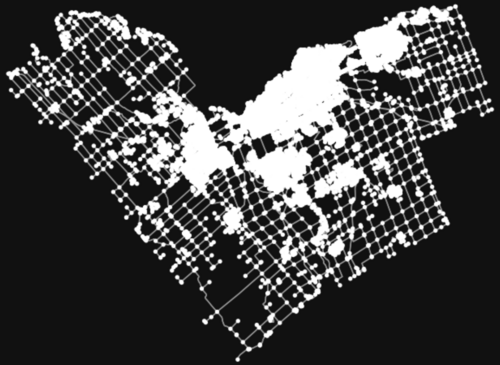
To explore some of the network analysis options in Python, this tutorial will use the road network of Ottawa, Ontario. This can easily be acquired using the OSMnx package, which uses Overpass API. The graph_from_place() function geocodes the area of interest (AOI) query and filters the network to the City of Ottawa's boundaries, while graph_from_polygon works with a custom polygon.
For additional information, check out the OSMnx documentation here and the example gallery here.
# create query for Smiths Falls
AOI = "Ottawa, Ontario, Canada"

# retrieve road network -> this may take some time
graph = osmnx.graph_from_place(
    AOI,
    network_type="drive" # this selects roads only. Other network options include "bike" and "walk".
)

# visualise the road network
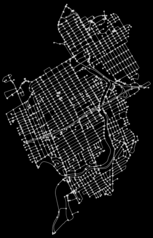
figure, ax = osmnx.plot_graph(graph)
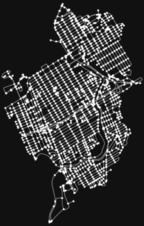
Let's pick a smaller area that is easier to visualise. A geojson boundary is provided below, but can be replaced with any custom polygon.
# Downtown boundary -> this can be replaced with any geodataframe
ott_boundary_geojson = {
"type": "FeatureCollection",
"name": "ott_boundary",
"crs": { "type": "name", "properties": { "name": "urn:ogc:def:crs:OGC:1.3:CRS84" } },
"features": [
{ "type": "Feature", "properties": { "id": 1 }, "geometry": { "type": "MultiPolygon", "coordinates": [ [ [
    [ -75.700646544981723, 45.442406206090276 ], [ -75.692602224956474, 45.439061352815521 ], [ -75.690143080492803, 45.436977332083586 ],
    [ -75.686975368980271, 45.436893971254314 ], [ -75.684016059540923, 45.438561187839852 ], [ -75.679535414967276, 45.437998502242237 ],
    [ -75.671449414527402, 45.433851300985694 ], [ -75.67046992478339, 45.42670310987517 ], [ -75.668531785502708, 45.424410687070051 ],
    [ -75.667531455551384, 45.42140969721607 ], [ -75.663592656368039, 45.418596269227969 ], [ -75.663092491392362, 45.415928722691106 ],
    [ -75.664426264660804, 45.414970073154414 ], [ -75.668406744258789, 45.414365707142153 ], [ -75.670657486649262, 45.413282016361556 ],
    [ -75.672199661990902, 45.412219165788272 ], [ -75.673095790905634, 45.410072624434378 ], [ -75.668740187575892, 45.404154005555696 ],
    [ -75.669865558771136, 45.400173525957719 ], [ -75.672783187795829, 45.397672701079401 ], [ -75.674429564174062, 45.3940048245912 ],
    [ -75.678014079832991, 45.389128216078483 ], [ -75.689069809815834, 45.383136656474207 ], [ -75.695373972529922, 45.381729942480156 ],
    [ -75.700063019176767, 45.378676852107873 ], [ -75.702199140426984, 45.378176687132189 ], [ -75.701886537317193, 45.381261037815442 ],
    [ -75.700094279487729, 45.383803543108399 ], [ -75.700531923841439, 45.387554780425873 ], [ -75.70151141358545, 45.392181306450752 ],
    [ -75.708805486147227, 45.396057585012137 ], [ -75.713369491550125, 45.403497539025139 ], [ -75.723758334898761, 45.410385227544161 ],
    [ -75.725748574697747, 45.418075264044965 ], [ -75.70428316115887, 45.425369336606728 ], [ -75.700646544981723, 45.442406206090276 ]
] ] ] } }
]
}

AOI = gpd.GeoDataFrame.from_features(ott_boundary_geojson["features"], crs="EPSG:4326")

# retrieve road network -> this may take some time
graph = osmnx.graph_from_polygon(
    AOI.geometry.iloc[0],
    network_type="drive" # this selects roads only. Other network options include "bike" and "walk".
)

# visualise the road network
figure, ax = osmnx.plot_graph(graph)
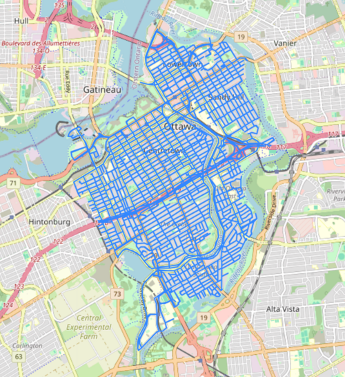
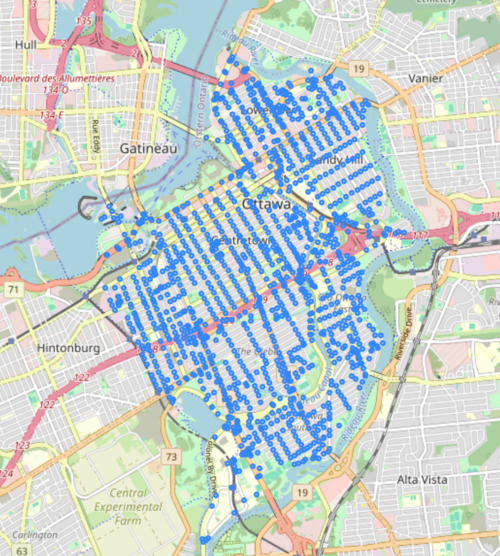
Let's examine the network with a basemap. We can do this by extracting the nodes and edges of the graph as geodataframes and using the .explore() method from GeoPandas.
# create geodataframes
nodes, edges = osmnx.graph_to_gdfs(graph)

# view edges with basemap
edges.explore()
# view nodes with basemap
nodes.explore()
Plot Customization
This looks good. Now let's customize some of the plotting parameters.
The configuration below can be easily applied as a base for any OSMnx plot we create later on.
Feel free to experiment!
Read the OSMnx documentation for further customization options.
# plot settings -> to be used as a base for most plots later on
pgr_args = {
    "figsize": (8, 10),           # figure size (width, height)
    "bgcolor": "black",          # background colour
    "node_color": "black",       # colour(s) of the nodes
    "node_size": 5,              # size(s) of the nodes
    "node_alpha": 1,             # opacity of the nodes
    "node_edgecolor": "white",   # colour(s) of the node borders
    #"node_zorder" : 0           # this will plot nodes under the edges
    "edge_color": "grey",        # colour(s) of the edges
    "edge_linewidth": 1,         # line width(s) of the edges
    "edge_alpha": 1,             # opacity of the edges
}

# plot graph with new settings
fig, ax = osmnx.plot_graph(graph, **pgr_args)
Projecting the Graph
Let's check the current coordinate reference system:
print(graph.graph['crs'])
epsg:4326
Data imported with OSMnx by default uses "EPSG:4326", which is the code for the WGS 84 Datum, a geographic coordinate system. For distance calculations, we need to use a projected coordinate system (x/y in meters).
Now we project the graph to the appropriate UTM zone and look at some basic statistics.
# project graph to UTM
crs = "EPSG:32618"
graph = osmnx.project_graph(graph, to_crs=crs)

# view basic statistics
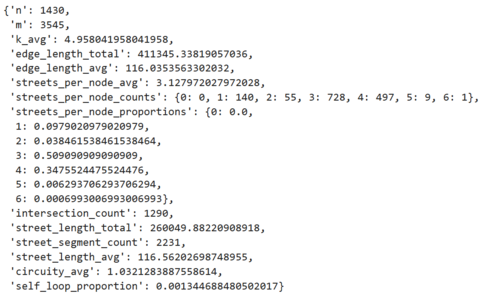
osmnx.basic_stats(graph)
This function shows some useful statistics about the graph. The first two lines show that there are 1430 nodes and 3545 edges. Note the difference between edge_length_total and street_length_total - remember that this a directed graph, with both single and bi-directional edges (roads). If every street was bi-directional, the the total street length should be exactly half of the total edge length. In this case, it is closer to 60%, which makes sense as Ottawa has a number of one-way streets and single direction highway ramps.
Check out the documentation for explanations of all the provided stats.
Simple Routing: Shortest Path
Let's explore one of the most basic applications of network analysis - determining the shortest path in the network between two nodes. This works the same way as a least-cost path analysis done on a raster, except with edges instead of pixels. A cost or weight is assigned to each edge, and an algorithm is used to calculate the path between two nodes with the lowest cumulative cost. OSMnx uses Dijkstra's algorithm.
See here more information on how Dijkstra's Algorithm works, as a great visualisation of how the algorithm works here.
For additional shortest path options not shown in this tutorial, see the NetworkX documentation.
Distance-Based
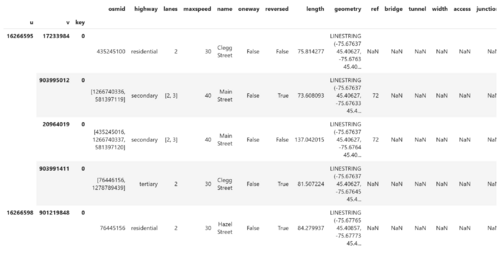
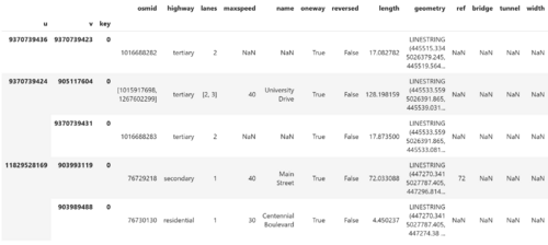
For a road network, the easiest cost or weight to use is distance. First, convert the graph into GeoDataFrames for nodes and edges. Exploring the edges geodataframe shows that distance is already present in the "length" column (this is done as part of the graph_from_place() function used earlier).
# extract gdfs
nodes, edges = osmnx.graph_to_gdfs(graph)

display(edges.head())
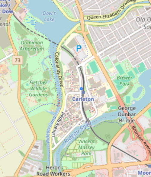
In this senario, a Carleton Student has just finished class and is going to pick up their friend from the athletics field at the University of Ottawa.
Let's define the start and end point using the geocoding functions in OSMnx. This can be done by simply querying the name of the building or place. However, it is not uncommon for the geocoding to fail, either because the feature is not present in the OSM data, or that the geocoding API requires that feature's name in a particular, sometimes unintuitive format. In this case, an address can be provided instead.
The geocoder outputs a geodataframe of the polygon feature (typically a building), but we need a point feature, so we take the centroid. It is also important to make sure that these new features use the same coordinate system as the graph.
# geocode start and end points, project to UTM and take centroid
start_point = osmnx.geocode_to_gdf("Carleton University, Ottawa").to_crs(crs).centroid
end_point = osmnx.geocode_to_gdf("Gee-Gees Field, Ottawa").to_crs(crs).centroid
We can quickly verify that the geocoding worked properly using the GeoPandas GeoDataFrame.explore() method.
start_point.explore()
end_point.explore()
Now we find the closest node in the network to the centroid points. This function outputs a list of nodes as it can be used for multiple input points, so the appropriate node IDs have to be converted to integers before proceeding.
# Find closest nodes
start_node = osmnx.nearest_nodes(graph, start_point.x, start_point.y)
end_node = osmnx.nearest_nodes(graph, end_point.x, end_point.y)

# convert to int -> for plotting
start_node = int(start_node[0])
end_node = int(end_node[0])
Let's determine the distance-weighted shortest path, with the weight set to the "length" column. The route can be plot using plot_graph_route, to which we can pass the plot configuration made earlier.
# Calculate a simple shortest path -> uses Dijkstra's Algorithm
route = osmnx.shortest_path(graph, start_node, end_node, weight='length')

# Plot the shortest path
fig, ax = osmnx.plot_graph_route(graph, route, orig_dest_size=100, **pgr_args)
OPTIONAL: Extracting Street Names
Now let's examine the roads taken by this route. The route_to_gdf() tool creates a geodataframe of only the edges traversed by this route. Because it is possible that the same road name appears multiple times, the aggregation must be done slightly differently than simply taking the unique names.
# create geodataframe of route
route_gdf = osmnx.routing.route_to_gdf(graph, route) # extracts edges used by route

# extract road names from
road_names = list(route_gdf.reset_index()['name'])

# aggregate road names
roads = []
for road_name in road_names:
    if not roads or roads[-1] != road_name:
        roads.append(road_name)

display(roads)
# filter edges in the route without street names
display(route_gdf[route_gdf['name'].isna()])
The "junction" column shows that this is part of a roundabout (the one by Carleton's main entrance), which doesn't have a street name in the OSM database.
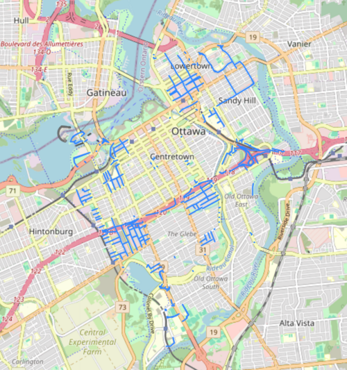
Let's explore the edges that are missing street names in the whole network.
# filter edges in the graph without street names
no_names = edges[edges['name'].isna()]
no_names.explore()
As expected, they mostly comprise slip lanes and some driveways and can be ignored.
Time-Based
While distance-weighted shortest paths may be useful for walking or biking networks, travel time is often more important for driving routes. First, we need to calculate the edge speeds, or speed limits for every road segment. Then, the edge travel time can be calculated from the speed and length of each edge. Finally, intersection impedences can be added to approximate time costs for stop signs and traffic lights.
Side note: The osmnx.elevation module allows for edge grades to be calculated, which may be useful for calculating travel time in walking and biking networks, though this is not covered in this tutorial.
Add Edge Speeds
Edge speeds represent the maximum speed of a given edge, in this case the speed limit for driving on a given road segment.
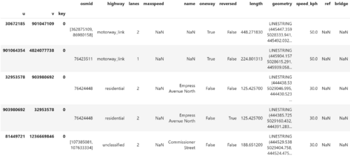
Fortunately, the OSM data already contains speed limits for most road segments, stored in the 'maxspeed' column.
# 'maxspeed' stores speed limits
display(edges)
As seen previously with the roundabout missing a road name, the OSM data is not perfect.
Let's investigate the edges with missing speed limits.
# filter edges in network that are missing 'maxspeed' values
no_maxspeed = edges[edges['maxspeed'].isna()]
no_maxspeed.explore()
The edges missing edge speeds include lot of small residential streets, driveways, slip lanes, and some highway ramps. Some areas are clearly more complete than others. For calculating travel time, we need every road segment in the network to have an edge speed.
OSMnx has a useful function for generating edge speeds based on the road classification (OSM highway tag).
- For example, a street with the "residential" tag will be assigned a value equal to the median of all "residential" segments that do have an edge speed.
# generate missing edge speeds
graph = osmnx.routing.add_edge_speeds(graph,
                                       hwy_speeds=None,  # existing values of the same highway type will be used to generate the speed (can be replaced with a custom dict.)
                                       fallback=40,      # if a highway type is not found or recognized
                                       agg=np.nanmedian) # median instead of mean to keep round numbers (30, 40, etc.)

# extract geodataframes again
nodes, edges = osmnx.graph_to_gdfs(graph)

# filter edges missing 'maxspeed' values
edges[edges['maxspeed'].isna()].head()
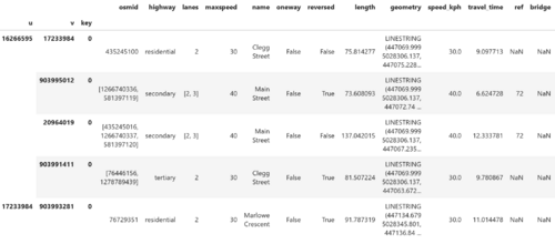
The 'speed_kph' column now contains any existing edge speeds from the 'max_speed' column as well as the values that were just generated.
Calculate Edge Travel Times
This is a simple calculation using the speed limit and length of each segment. OSMnx has a useful function that automatically creates a new column "travel_time" with the time in seconds.
# calculate travel time
graph = osmnx.routing.add_edge_travel_times(graph)

# extract geodataframes
nodes, edges = osmnx.graph_to_gdfs(graph)

edges.head()
Add Intersection Impedances
The travel times we calculated earlier represent edge impedances, but there may also be impedances over nodes, especially in cities where there are many intersections with traffic lights. OSM uses tags to represent different types of intersections, so these can be used to generate average time costs at traffic lights and stop signs.
nodes.head()
It looks like a lot of nodes don't have tags. This makes sense, as not all nodes are intersections, and some intersections may not be signaled or signed. As we saw earlier with road names and edge speeds, the OSM data can be incomplete, so this warrants a closer look.
# calculate percentage of nodes without intersection data
print(len(nodes[nodes['highway'].isna()])/(len(nodes))*100)

# View of all nodes (intersections) without a tag (traffic lights, stop sign, etc.)
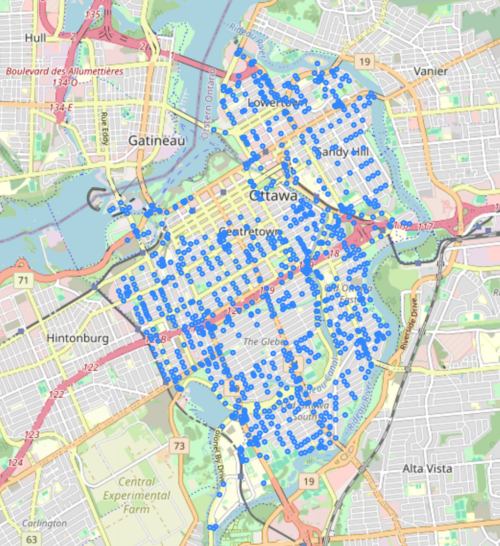
nodes[nodes['highway'].isna()].explore()
68.74125874125873
Almost 70% of the nodes in this area are missing a tag. Similar to the edge speeds, some areas are much more complete than others. While there was an easy way to fill in the missing edge speeds, there isn't a simple way to fix this issue, so unfortunately we will have to leave out intersection impedances from our time-weighted shortest path for Ottawa.
Time-Based Shortest Path
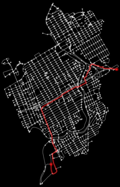
Let's try calculating the shortest path again, this time using travel time as the weight.
# Calculate a simple shortest path -> uses Dijkstra's Algorithm
route2 = osmnx.shortest_path(graph, start_node, end_node, weight='travel_time')

# Plot the shortest path
fig, ax = osmnx.plot_graph_route(graph, route2, **pgr_args)
OPTIONAL: Extracting Street Names
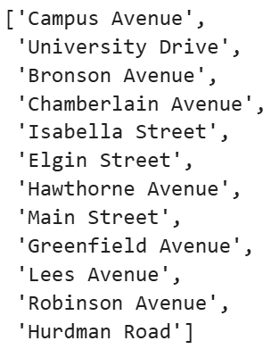
The second route takes a different path. Let's explore the road names again, but this time we can ignore any missing names, which we determined to only be slip lanes, driveways, and highway ramps.
# export road names from route
route_gdf = osmnx.routing.route_to_gdf(graph, route2) # extract this route's edges (road segments) from the larger network

road_names = list(route_gdf.reset_index()['name'])

# Because the same road name may appear multiple times, the aggregation must be done slightly differently than simply finding the unique names.
roads = []
for road_name in road_names:
    if pd.isna(road_name): # ignore edges without road names -> highway ramps and slip lanes
        continue
    if not roads or roads[-1] != road_name:
        roads.append(road_name)

display(roads)
