Digitizing in Python

Purpose

The purpose of this tutorial is to automate the digitization of land cover features such as vegetation, waterbodies, and roads, using Sentinel-2 satellite imagery and Python-based geospatial tools.

Objective

Use Google Earth Engine (GEE) to acquire the satellite images for processing in python. Compute NDVI (vegetation), NDWI (water), NDBI (roads) indices. Export rasters to your Google Drive. Convert rasters to vectors. Visualize and colourize digitized features.

Software Used

Google Earth Engine Google Colab or any other Python language system or notebooks.

Python libraries:

 earthengine-api, geemap, rasterio, geopandas, shapely, matplotlib

Setting up Colab and Google Earth Engine

Set up a Google Earth Engine account for free with these similar instructions (note that you do not need to make an account under a student requirement or the sort or any paid service, this is free!): https://courses.spatialthoughts.com/gee-sign-up.html

After your account is created, create a new project under a name of your choice. This will be linked back in the Colab notebook.

To set up a Colab notebook, simply open a new Colab notebook within your Google Drive.

Now, in the Colab notebook, follow this code and replace the project name with your own project name from when you created a project in Google Earth Engine in the code snippet below:

 
!pip install earthengine-api geemap rasterio geopandas shapely matplotlib

import ee
import geemap
import geopandas as gpd
from shapely.geometry import shape
import matplotlib.pyplot as plt
import numpy as np
from rasterio.features import shapes
import rasterio
from rasterio.plot import show

ee.Authenticate()
ee.Initialize(project='your-project-name')

Note that when you run the code above in Colab, a pop-up asking for permission for Colab to authorize the use of third-party notebook code will appear. You can accept this.

What is Digitizing?

Digitizing is the process of converting geographic features into digital vector forms. Though this used to be a manual process using different techniques by hand, it can be done in a digital space or even automated using indices and raster-to-vector conversion.

Why is Digitizing Important?

Digitizing geographic data is crucial for converting analog maps and spatial information into a digital space because digital formats are preferred, with the ability to be easily analyzed, shared and constantly up to date.

Data

• Sentinel-2 imagery from Google Earth Engine
• Area of Interest: Hogsback River near Carleton University

Choosing Your Own Satellite Image

The code below is based on the coordinate data of Hogsback River, near Carleton University. Any area in the world within the limits of what satellite images Google Earth Engine has access to can be used in place of the chosen coordinates for this tutorial.

 
aoi = ee.Geometry.Point([-75.6909, 45.3795])  # longitude, latitude
aoi_buffer = aoi.buffer(1000).bounds()        # 1 km buffer around the river

Methods

The main method is using NDVI, NDWI, and NDBI and setting up these bands to represent them in the output images as well as setting up a threshold value for each.

Spectral Indices

Index	Purpose	Bands Used	Threshold
NDVI	Vegetation	B8, B4	0.3
NDWI	Waterbodies	B3, B8	0.2
NDBI	Built-up Roads	B11, B8	0.2

Steps

Part 1: Getting Started

This part follows some required loading of the sentinel imagery, such as cloud coverage settings, threshold value for vegetation only, setting the time frame and what it the final map in part 2 will resemble. Once you have loaded the area of interest, the next step is to select the parameters for time, cloudiness percentage, and to see what the final output will look like.

Step 1

Selecting filters for the image and library from Copernicus Sentinel-2 imagery:

 
collection = (ee.ImageCollection("COPERNICUS/S2_SR")
              .filterBounds(aoi_buffer)
              .filterDate("2024-06-01", "2024-08-31")  # summer imagery
              .filter(ee.Filter.lt("CLOUDY_PIXEL_PERCENTAGE", 10)))

Step 2

Select least cloudy image:

 
image = collection.sort("CLOUDY_PIXEL_PERCENTAGE").first()

Step 3

Compute NDVI (this is just to see a third of what the output will resemble):

 
ndvi = image.normalizedDifference(["B8", "B4"]).rename("NDVI")

Step 4

Selecting parameters to display the map:

 
Map = geemap.Map()
Map.centerObject(aoi_buffer, 13)
Map.addLayer(image, {"bands":["B4","B3","B2"], "min":0, "max":3000}, "Sentinel-2 RGB")
Map.addLayer(ndvi, {"min":0, "max":1, "palette":["white","green"]}, "NDVI")

Step 5

Saving the raster to the Google Drive:

 
task = ee.batch.Export.image.toDrive(
    image=ndvi,
    description="Hogsback_NDVI",
    folder="EarthEngine",
    fileNamePrefix="hogsback_ndvi",
    region=aoi_buffer.getInfo()['coordinates'],
    scale=10,
    crs="EPSG:4326"
)
task.start()
print("Export started. Check Google Drive → EarthEngine folder for hogsback_ndvi.tif")

Step 6

Mount Google Drive in Colab once the export finishes:

 
from google.colab import drive
drive.mount('/content/drive')

Note that in doing the code above, another pop-up will open for permission for your Google Drive to be connected to Colab. You can, of course, accept.

Step 7

Load the raster locally with Rasterio. (Note that the filepath will look different depending on where you have it saved in your drive):

dataset = rasterio.open("/content/drive/My Drive/EarthEngine/hogsback_ndvi.tif")
ndvi_array = dataset.read(1)

Step 8

Apply threshold for vegetation:

mask = ndvi_array > 0.3

Step 9

Raster to vector:

results = (
    {"properties": {}, "geometry": shape(geom)}
    for geom, val in shapes(ndvi_array.astype(np.int16),
                            mask=mask,
                            transform=dataset.transform)
)

gdf = gpd.GeoDataFrame.from_features(results, crs=dataset.crs)

Step 10

Export the digitized polygon:

gdf.to_file("hogsback_digitized_vegetation.shp")

Step 11

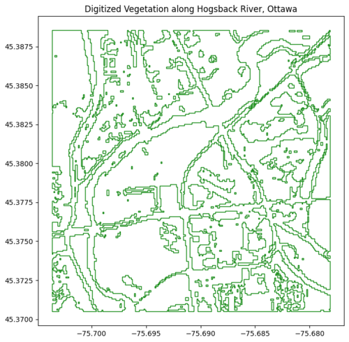
Visual of the map:

fig, ax = plt.subplots(figsize=(8,8))
gdf.plot(ax=ax, facecolor="none", edgecolor="green")
plt.title("Digitized Vegetation along Hogsback River, Ottawa")
plt.show()

If you did the area of interest seen in the previous section of this tutorial (area in Hogsback Falls near Carleton) your output should look something like this:

(if you got nothing, you may need to adjust the time frame as there may not be an image available for that area and maybe adjust the cloud coverage settings).

Part 2: The Full Process

In this part, the full process is applied or continued by adding water and road data into the previous map, along with vegetation.

Step 1

Import another library called time, it will be used for polling:

import time

Step 2

Now compute NDVI, NDWI, NDBI from Sentinel-2 imagery:

ndvi = image.normalizedDifference(["B8", "B4"]).rename("NDVI")
ndwi = image.normalizedDifference(["B3", "B8"]).rename("NDWI")
ndbi = image.normalizedDifference(["B11", "B8"]).rename("NDBI")

Step 3

Export each raster into your Drive:

export_tasks = []
for index, name in zip([ndvi, ndwi, ndbi], ["ndvi", "ndwi", "ndbi"]):
    task = ee.batch.Export.image.toDrive(
        image=index,
        description=f"Hogsback_{name.upper()}",
        folder="EarthEngine",
        fileNamePrefix=f"hogsback_{name}",
        region=aoi_buffer.getInfo()['coordinates'],
        scale=10,
        crs="EPSG:4326"
    )
    task.start()
    export_tasks.append(task)
    print(f"Export started for hogsback_{name}.tif. Task ID: {task.id}")

Step 4

Wait for all tasks to finish with polling:

print("\nWaiting for all Earth Engine exports to complete...")
for task in export_tasks:
    # Poll task status until it's not 'READY' or 'RUNNING'
    while task.status()['state'] in ['READY', 'RUNNING']:
        print(f"Task '{task.status()['description']}' is {task.status()['state']}, waiting...")
        time.sleep(10) # Wait for 10 seconds before checking again

    if task.status()['state'] != 'COMPLETED':
        raise Exception(f"Export task failed for {task.status()['description']}: {task.status()['error_message'] if 'error_message' in task.status() else 'Unknown error'}")
    print(f"Export task '{task.status()['description']}' completed.")

Step 5

After the export is done, load rasters locally with Rasterio (your filepath may look different here):

dataset_ndvi = rasterio.open("/content/drive/My Drive/EarthEngine/hogsback_ndvi.tif")
dataset_ndwi = rasterio.open("/content/drive/My Drive/EarthEngine/hogsback_ndwi.tif")
dataset_ndbi = rasterio.open("/content/drive/My Drive/EarthEngine/hogsback_ndbi.tif")

ndvi_array = dataset_ndvi.read(1)
ndwi_array = dataset_ndwi.read(1)
ndbi_array = dataset_ndbi.read(1)

Step 6

Apply threshold to NDVI, NDWI, NDBI:

veg_mask = ndvi_array > 0.3
water_mask = ndwi_array > 0.2
road_mask = ndbi_array > 0.2

Step 7

Convert each mask to polygons. Here, we also make rules to return the output if no polygons are found and will return an output with an empty geometry column:

def raster_to_polygons(array, mask, transform, crs):
    # Convert generator to list to check if it's empty
    features_list = [
        {"properties": {}, "geometry": shape(geom)}
        for geom, val in shapes(array.astype(np.int16), mask=mask, transform=transform)
    ]
    if not features_list:
        # If no polygons were found, return an empty GeoDataFrame with a geometry column
        return gpd.GeoDataFrame(geometry=[], crs=crs)
    return gpd.GeoDataFrame.from_features(features_list, crs=crs)

veg_gdf = raster_to_polygons(ndvi_array, veg_mask, dataset_ndvi.transform, dataset_ndvi.crs)
water_gdf = raster_to_polygons(ndwi_array, water_mask, dataset_ndwi.transform, dataset_ndwi.crs)
roads_gdf = raster_to_polygons(ndbi_array, road_mask, dataset_ndbi.transform, dataset_ndbi.crs)

Step 8

Filter the polygons:

veg_gdf = veg_gdf[veg_gdf.area > 1000]
water_gdf = water_gdf[water_gdf.area > 500]
roads_gdf = roads_gdf[roads_gdf.area > 200]

Step 9

Here we save the shapefiles using rules again:

if not veg_gdf.empty:
    veg_gdf.to_file("hogsback_vegetation.shp")
else:
    print("No vegetation polygons to save after filtering.")

if not water_gdf.empty:
    water_gdf.to_file("hogsback_waterbodies.shp")
else:
    print("No waterbody polygons to save after filtering.")

if not roads_gdf.empty:
    roads_gdf.to_file("hogsback_roads.shp")
else:
    print("No road polygons to save after filtering.")

Step 10

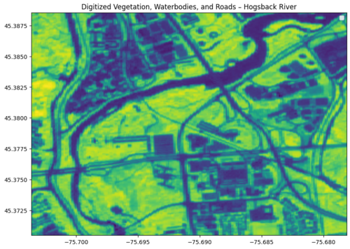
Visualizing the final map with a final rule that makes it so that if each one is not empty, it will show on the map with specific colours (colours can be modified for your disclosure):

fig, ax = plt.subplots(figsize=(10,10))
show(dataset_ndvi, ax=ax)

# Plot only if GeoDataFrame is not empty
if not veg_gdf.empty:
    veg_gdf.plot(ax=ax, facecolor="none", edgecolor="green", label="Vegetation")

if not water_gdf.empty:
    water_gdf.plot(ax=ax, facecolor="blue", edgecolor="blue", alpha=0.5, label="Water")

if not roads_gdf.empty:
    roads_gdf.plot(ax=ax, facecolor="gray", edgecolor="black", alpha=0.5, label="Roads")

plt.legend()
plt.title("Digitized Vegetation, Waterbodies, and Roads – Hogsback River")
plt.show()

Should come out looking something like this (May take 2-3 minutes for processing):

Conclusion

This tutorial shows how to do a complete digitization of an area in Google Colab using Python alongside Google Earth Engine for Sentinel-2 satellite images. By automating the process of spectral classification and vectorizing the images, land cover features can be extracted for environmental analysis. This process is reproducible and can be adapted to other areas of interest.

References

Sign-up for Google Earth engine. (n.d.). https://courses.spatialthoughts.com/gee-sign-up.html

Google Earth Engine. (n.d.). https://earthengine.google.com/

Rasterio: access to geospatial raster data — rasterio 1.4.4 documentation. (n.d.). https://rasterio.readthedocs.io/en/stable/

GeoPandas 1.1.1 — GeoPandas 1.1.1+0.ge9b58ce.dirty documentation. (n.d.). https://geopandas.org/en/stable/

Shapely — Shapely 2.1.2 documentation. (n.d.). https://shapely.readthedocs.io/en/stable/

Matplotlib — Visualization with Python. (n.d.). https://matplotlib.org/