Fire Risk Analysis using QGIS

NOTE: This is a work in progress, and subject to change.

Purpose

This tutorial will demonstrate how to use multiple tools within QGIS in order to perform a fire risk analysis. This analysis includes manipulating vector and raster data in order to produce final output maps. This tutorial uses tools from QGIS' advanced interface, which include QGIS, GRASS GIS, and plugins that will require an internet connection in order to download them into QGIS. Major tools that will be used in this tutorial include:

Build Virtual Raster Catalog - QGIS

Clipper - QGIS

Merge Vector Layers - QGIS

Polygonize - QGIS

Rasterize - QGIS

Raster Calculator - QGIS

Aspect and Slope - GRASS GIS

Reclass - GRASS GIS

Heatmap - Plugin

Multi-distance Buffer - Plugin

Although this tutorial is a walk through, it is highly recommended that you have GIS knowledge before attempting this analysis.

Introduction

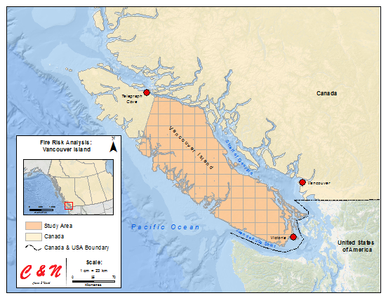
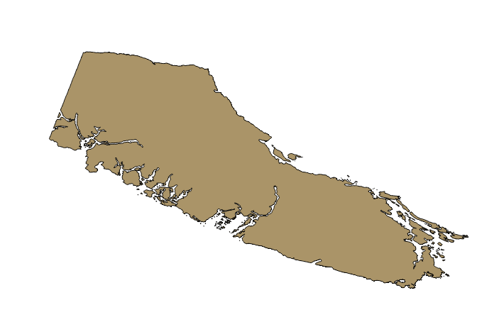
For the purpose of this tutorial, the study area that will be used to demonstrate a Fire Risk Analysis will be approximately 75% of Vancouver Island from just South of Telegraph Cove to Victoria (Figure 1). During this fiscal year (April 1, 2015 – March 31, 2016) there have been 1 843 fires in the entire province of British Columbia which has resulted in approximately 305 000 hectares of land being burned. The area that we will be analyzing for the purpose of this tutorial around Vancouver Island has had just under 200 fires resulting in approximately 25 000 hectares of burnt land according to the Government of B.C. Wildfire Service.

This tutorial will demonstrate how to create maps that identify areas that have a high risk of fires based on multiple factors. These maps in turn, can help respondents react quicker to help prevent future fires by implementing measures based on the high risk of fires in a certain area of the island. This analysis is based on summer months in British Columbia (Landsat Imagery acquired from the end of June 2013).

The way risk will be calculated evenly for the purpose of this analysis will be from 1 to 4. With 1 being the lowest possible risk, and 4 being the highest possible risk. This will be accomplished by using reclassification methods.

1 = Low Risk

2 = Moderate-Low Risk

3 = Moderate-High Risk

4 = High Risk.

All data and software used in this tutorial are open-sourced and can be found online.

Figure 1: The study area for this tutorial is shown here as a pink grid feature, from just south of Telegraph Cove to Victoria.

Software

The software being used for this tutorial is a Geographic Information System named QGIS formerly known as Quantum GIS. You can download the software by clicking here.Select the appropriate file to download onto your computer and follow the download instructions after that. QGIS can be downloaded and used on many different operating systems including; Android, BSD, Linux, Mac and Windows. QGIS updates its versions often, for our specific tutorial we used QGIS version 2.8, if you attempt this tutorial in the future some features may be different.

Once you have downloaded the software, you may begin the tutorial.

Data

Data Identification

In order for the analysis to be run, data sets were identified based upon research of academic journals and research papers which topics included a fire risk analysis, assessment or use of a GIS with forest fires. Based upon the research, the 5 major data sets that were needed include:

1. Census subdivisions & attribute data (population density)

2. Landsat 8 imagery (Normalized Difference Vegetation Index - NDVI)

3. Digital Elevation Model (aspect and slope - DEM)

4. Past wildfires (spatial pattern/clustering)

5. Mitigation factors (bodies of water)

The data sets were then categorized into three different categories (Table 1), which will create three maps that will be calculated against each other; fire hazards, vulnerability factors & mitigation factors.

Table 1. Data sets that were collected, categorized into three different categories.

Data Set Links & Guide

1. Census Subdivisions Attribute Data Attribute Data *

Download the census subdivision boundary file as a shapefile and download the census subdivision attributes.

2. Landsat 8 Imagery **

Once you have created an account, under Search Criteria select the area of your interest by creating a polygon around your study area. Select an appropriate date range, in our analysis we looked at data sets from July 2014 to August of 2014 when forest fires are most prominent in this region. Next, click Data Sets navigate to Landsat Archive, check the first box under that folder titled L8 OLI/TIRS. Under Additional Criteria you may select whether the imagery was taken during day or night and the percentage of cloud cover in the imagery. For the purpose of this tutorial, it would be ideal to select imagery during the day and with less than 10% cloud coverage. After all of these steps are completed your data sets should appear and you can now select the appropriate imagery to download. Note, you will have to unzip the files after they have downloaded in order to access the bands.

3. Digital Elevation Model

Simply pan the globe to your study area, click the tile and download. The elevation model is at a 90-metre resolution. Note, you will have to unzip the files after they have downloaded in order to access the elevation models.

4. Past Fires

Download the KMZ files from 2010 - 2014 (three separate files). QGIS will not be able to open a KMZ file, it is essentially a zipped KML file. You will have to unzip the KMZ file in order to get it into a KML which QGIS will be able to read and import.

5. Water Bodies

Download the zipped folder containing multiple shapefiles of British Columbia, after you have unzipped the folder the shapefile that will be needed for the analysis will be called, waterways.shp.

* Must be a Carleton University alumni, faculty, student or other institution approved by CHASS in order to access this attribute data.

** In order to access the Level 1 data that includes the bands needed to calculate the NDVI, you must create a USGS account.

Note: It is recommended you download 7-Zip to help unzip the Landsat Imagery and KMZ files.

Tutorial

Setting up the Environments

There are three steps in order to set up your environment for this tutorial.

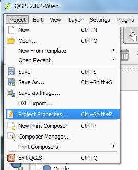
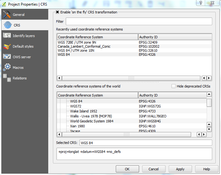
1. The first thing to do after opening the QGIS desktop, navigate to the Project tab and select Project Properties (Figure 2). This is where you can name your project (General Tab) and ensure your coordinate system is correct (CRS Tab). Under the CRS Tab, check 'Enable on the fly CRS transformation', and choose an appropriate coordinate reference system. We chose a WGS 84 (ESPG:4326).

Figure 2. Opening the properties tab to name your project and define an appropriate coordinate system for your study area, by enabling 'on the fly projection'. Here a WGS 84 coordinate system was used.

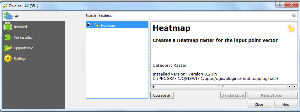
2. The next step will be to add the two plugins you will need for some analyses. Navigate to the Plugin tab (ensure you have internet connection) and select Manage and Install Plugins. The plugin interface will now appear. In the search box located at the top, type in heatmap and check the box beside the heatmap plugin (Figure 3) and also type in multi-ring buffer and check the plugin on. The heatmap tool creates a (raster) based on the proximity of vector points to one another, detecting spatial pattern/clustering which will be used for the past fires data. While the multi-ring buffer will be used for the water polylines, creating multiple buffers around the water features based on distances defined by the user.

Figure 3. Setting up the heatmap plugin needed in order to create a heatmap for the past fires points.

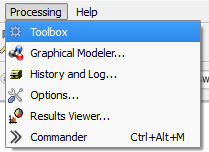
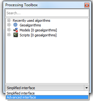
3. The final step in setting up your environment is to turn on the adavnced interface for your toolbox in order to access the GRASS GIS tools. Navigate to the Processing tab and select Toolbox and the toolbox interface should appear, and at the bottom of the toolbox Simple Interface should be on, click that box and turn Advanced Interface on (Figure 4).

Figure 4. Setting up the advanced toolbox interface.

Importing the Data

Since we have multiple types of data to be imported, we will have to use the Add Vector Layer and Add Raster Layer , located along the left hand-side of the QGIS user interface.

The data to be imported using the Add Vector Layer includes the following; Census subdivision cartographic boundary shapefile, three past fires kml files, and the waterways shapefile.

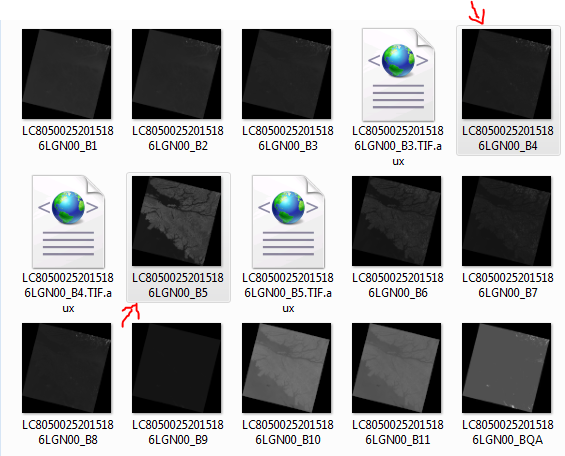
The data to be imported using the Add Raster Layer includes the following; Three Digital Elevation Models tiff files, and the three Landsat 8 Imagery tiff files. In order to calculate the NDVI, we will need the Red (4) and Near Infrared (5) bands, they will both need to be selected per imagery (Figure 5).

Figure 5. Importing the Red and Near Infrared bands per imagery, in order to calculate NDVI.

Organizing the Data

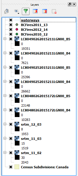
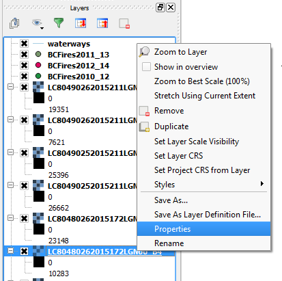
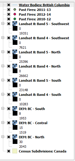
In order to keep your data organized, and to avoid confusion it is a good idea to group your data based on the five data types that were imported. After importing the data it will look quite messy and may not make much sense, so it is recommended that you change the name of the data immediately after importing to a name that makes sense or relates to set data layer. In the layer on the left hand-side right click your data, click properties and rename your data for each - it is recommended you do this for each data set imported. (Figure 6)

Figure 6. The figures showing the messiness of data, along with renaming and the ideal layer renaming scheme.

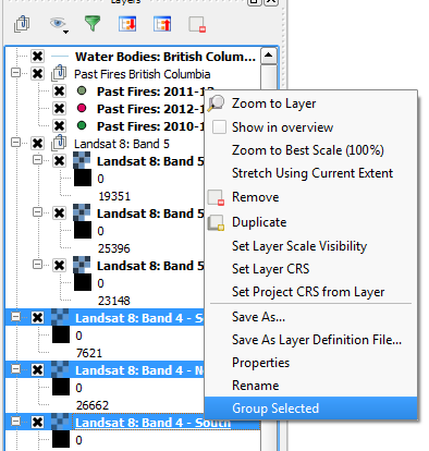
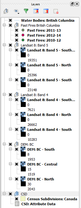
The next step is to group the data based on the original 5 categories that the data were imported in, as depicted in Figure 7. Hold the control button on PC or command on Mac and select the appropriate data layers to group, right click and select group and rename accordingly.

Figure 7. The figures show how to group the data along with the ideal grouping scheme.

Working with the Data

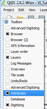
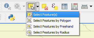
Now we can begin to use tools to manipulate the data. We first need to work with the Census subdivision (CSD) boundary shapefile to create a CSD of Vancouver Island. However, this will not be our area of interest. In order to create a new shapefile of just Vancouver Island you must turn the attribute toolbar on, it should be automatically turned on - if it is not right click just under the properties and check the attribute toolbar on. After you have done so, move to select features (it can be done by polygon, freehand, etc. - whatever you feel most comfortable with) and select all census subdivisions that reside on Vancouver Island (Figure 8).

Figure 8. This figures demonstrates how to turn on the attribute toolbar and select features in order to create the new shapefile.

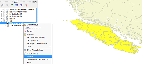
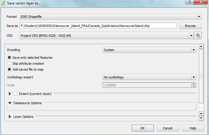
After you select the method you wish to select features with, in the case shown with Figure 9 hold control or command while selecting the polygons. After all features are selected, right click the CSD layer and save the selected features as a new shapefile, give it an appropriate name.

Figure 9. The figures show Vancouver Island being selected and how to save the selected features as a new shapefile.

Creating an Area of Interest & Building Virtual Raster Catalogs

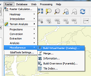
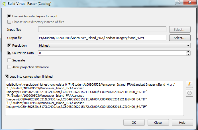
In order to create our area of interest we will need to build virtual rasters based on the Landsat imagery and clip it to the newly created Vancouver Island CSD shapefile. The first step is to turn all of your Landsat 8 imagery on (either all of the band 4 or band 5 imagery), then navigate to the Raster tab, click Miscellaneous and finally click Build a Virtual Raster (VRT). For all of the rasters imported you will need to create a virtual catalog for each group. Turn the group on that you wish to convert into one raster; you will need to do it for the Landsat 8 Imagery: Band 4, Landsat 8 Imagery: Band 5 and the three Digital Elevation Models. While creating the virtual raster (VRT), ensure that no data is set to 0 and the resolution is set to highest, these rules can be applied to all of the above (Figure 10).

Figure 10. These figures show how to create a Virtual Raster (VRT), and the rules can be applied to all of the raster data sets.

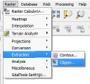
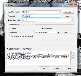
After the Virtual Rasters are created, you will want to clip it to just Vancouver Island. For this we will use the Band 4 VRT, navigate to the Raster tab, click Extraction and use the Clipper tool, use input Band 4 as the raster to be clipped and use the Vancouver Island shapefile as the mask layer. Ensure that no data is set to 0 (Figure 11).

Figure 11. The figures showing how to use the clipper tool, using band 4 as the raster, Vancouver Island as the mask layer and setting 0 as no data and the newly created band 4.

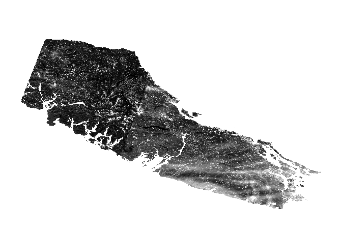
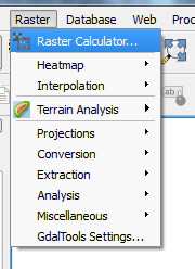
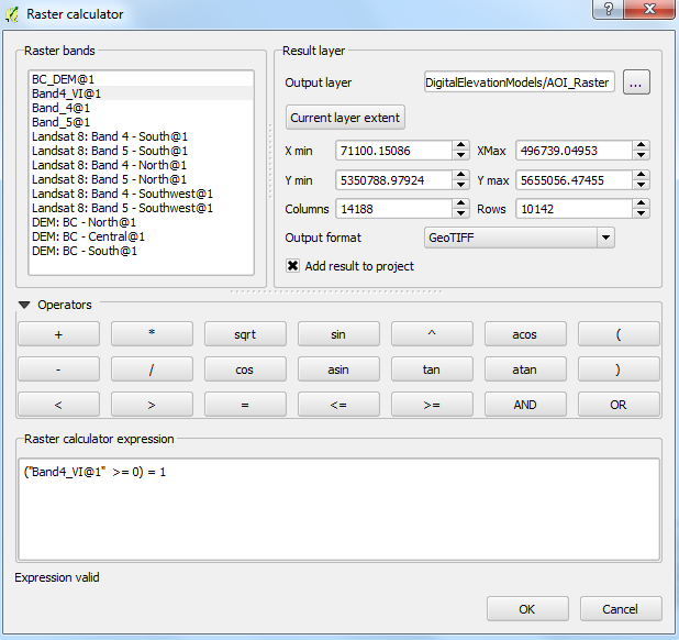
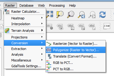
After using the clipper tool and creating the new band 4 raster, you will want to reclassify all the values to 1 in order to create the area of interest. Navigate to Raster and click Raster Calculator and all values that are greater than and/or equal to 0 shall equal 1. After this has been created you will want to create a polygon based on this value which will be your area of interest/study area, by using the Polygonize function that is located under Raster tab and Conversion (Figure 12).

Figure 12. These figures show how to use the raster calculator to create a simple reclassification (all values that are equal and/or greater than 0 equal 1), which was then converted to a polygon for the area of interest.

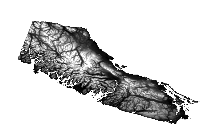
After successfully creating your area of interest/study area. You can again apply the Clipper function to the other two VRT created using the area of interest shapefile as your mask (Figure 13).

Figure 13. The figures above show Band 5 (top) and the Digital Elevation Model (bottom) clipped to the study area.

Calculating Normalized Difference Vegetation Index and Reclassification

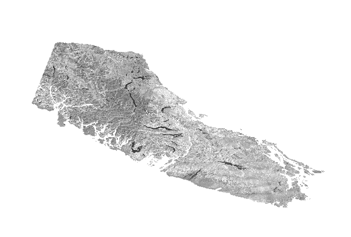
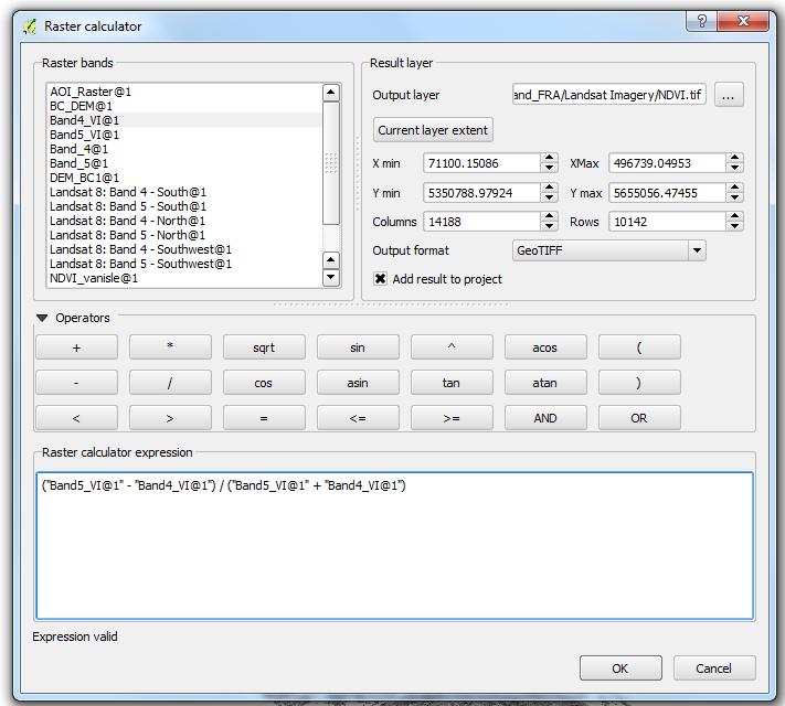
For this part of the tutorial, we will be using the raster calculator which was touched upon in the previous section in order to create a Normalized Difference Vegetation Index (NDVI). The reclassifying portion is where we first see the GRASS GIS tools being applied. The data that will be used in this section will be the newly clipped Band 4 (Red) and newly clipped Band 5 (NIR). A NDVI calculation requires the following: NDVI = NIR - RED / NIR + RED.

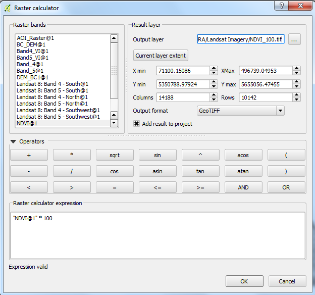
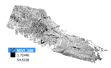
Using the raster calculator we will be able to do this calculation, the output values could/should range from -1.0 to 1.0. The reclassification tool from GRASS GIS has a difficult time reclassifying decimals and usually rounds up. So in order to reclassify more accurately, you will have to multiple the NDVI created by an appropriate value and then reclassify. We chose to multiply it by 100 (Figure 14).

Figure 14. The original NDVI calculation, the NDVI calculation multiplied by 100 in order for reclassification and the output values & visualization map.

Based on the values outputted by the last raster calculation, we now can reclassify based upon those values. Justification for the reclassification is as follows;

please refer to introduction for definition of risk numbers #Introduction

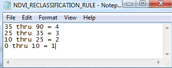
35 to 90 = 4

25 to 35 = 3

10 to 25 = 2

0 to 10 = 1

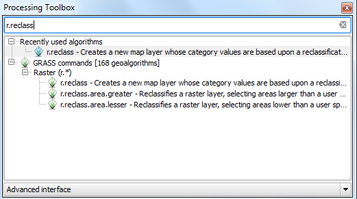
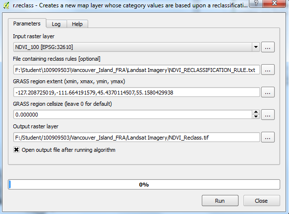
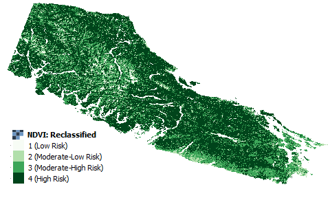
Now navigate to the advanced toolbox interface that we set up in section 5.1, type in r.reclass and open the tool. Choose the appropriate raster for reclassification, in this case the raster that was multiplied by 100. You will notice that it requires a text rule, simply open any word processor - Notepad is always quite easy to work with. Open the word processor and type in the justification above use thru instead of to (click here for more reclassification rules), save it as a .txt file, input it into the tool and run the process and you should have reclassified your NDVI which will await further calculations (Figure 15).

Figure 15. The above figures show where to find the reclassification tool, how to reclassify using a text file along with using the tool and finally the output from the reclassification.

Aspect, Slope and Reclassification

In this section we will be using the DEM that we clipped to our area of interest to preform aspect and slope analyses. Aspect is the compass direction slope is facing, and output generated usually represents degrees from 0 to 360 and will help us determine which way the wind traverses on land, where Slope is incline/steepness of the surface and the output generated usually represents degrees from 0 (Flat) to 90 (Straight up), the steepness of the slope affects both the rate and direction of the fire spread. Fires usually move faster uphill than downhill and the steeper the slope, the faster the fire will move. (1)

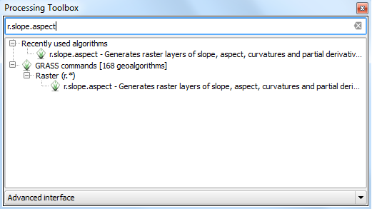
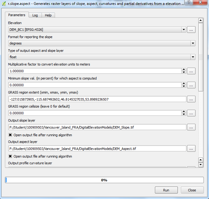
To create the Aspect and Slope rasters we will use the grass tool called r.slope.aspect which can be found in the advanced interface toolbox, after you have opened the tool input your DEM that was clipped to your area of interest, and give appropriate names to your aspect and slope models. If you scroll further down on the tool, you will notice it outputs many other types of terrain analyses - however they will not be needed for our overall analyses, so turn all the boxes off except for aspect and slope, run the tool (Figure 16).

Figure 16. Type in r.slope.aspect in the advanced interface toolbox, and input all of the necessary components in order to run the analyses.

The next step will be to reclassify the aspect and slope rasters just created. Since Westerly winds prevail over Vancouver island (2) aspect that faces east have the highest risk for this analysis, the justification for slope is as follows:

0 to 23 = 2 (North)

23 to 68 = 3 (Northeast)

68 to 113 = 4 (East)

113 to 158 = 3 (Southeast)

158 to 203 = 2 (South)

203 to 248 = 1 (Southwest)

248 to 293 = 1 (West)

293 to 338 = 1 (Northwest)

338 to 360 = 2 (North)

Now use the same methods for slope, slope in degrees with greater than or equal to 35 has high risk, the justification for slope reclassification is as follows;

0 to 10 = 1

10 to 25 = 2

25 to 35 = 3

35 to 90 = 4

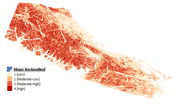
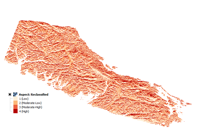
After both have been inputted into a .txt file, exactly like the processes in section 5.6 #Calculating_Normalized_Difference_Vegetation_Index_and_Reclassification, open r.reclass input your aspect raster and reclassification rule and run the tool, do the same for slope. The output maps should look similar to the figures in Figure 18.

Figure 18. Slope and Aspect Maps after reclassification and change of symbology.

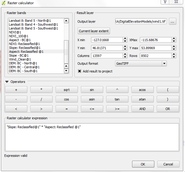
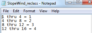
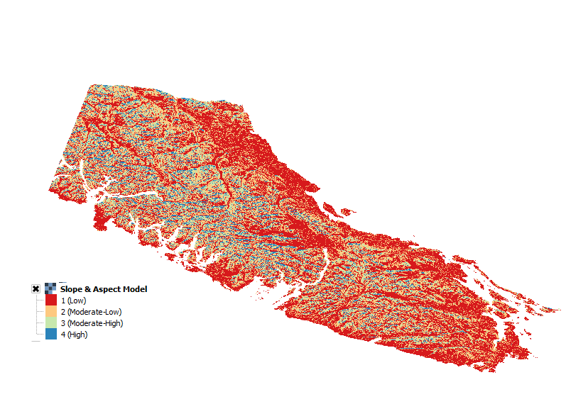
In order to create the output that will be used in the hazard calculation, we will need to combine aspect and slope to identify areas that face east and have high slope values associated with it, we will use the Raster Calculator in order to complete the process. Multiply both rasters by each other, and since both reclassified rasters have maximum values of 4 the maximum output value of the new raster map (we called it wind) will be 16. This can then be reclassified by using r.reclass and you will have your aspect and slope output (Figure 19), the reclassification scheme follows;

1 to 4 = 1

4 to 8 = 2

8 to 12 = 3

12 to 16 = 4

Figure 19. Map for reclassified slope and aspect calculation, then the reclassification scheme for the newly created raster and the final output of the wind raster which will be used in the final calculation.

Spatial Pattern and Heatmap of Past Fires

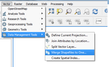
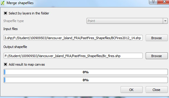
Using the three past fires point shapefiles, we must merge them together. In order to complete this process we will have to merge all the past fire point shapefiles in order to create the points we will use to create a heatmap. We will use the Merge Shapefiles to One tool, which is located under the Vector tab and located within the Data Management tab. Merge all of the point shapefiles located under a single directory (Figure 20).

Figure 20. The merge tool, in order to combine all past fire points to one.

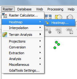
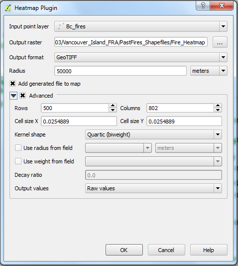
After this we can then use the heatmap plugin that we installed during the beginning of this tutorial which is located in the Raster tab, you will input the newly created shapefile of the three merged past fires point that you just completed and create a heatmap based upon the clustering of points, for the purpose of this tutorial create a radius of approximately 50 000 metres (Figure 21).

Figure 21. Location of the heatmap tool and parameters that will be used for this analysis.

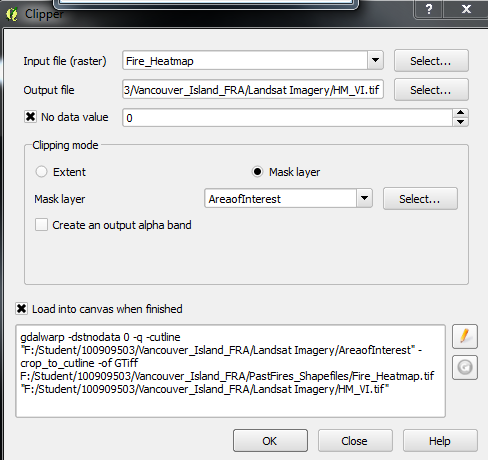
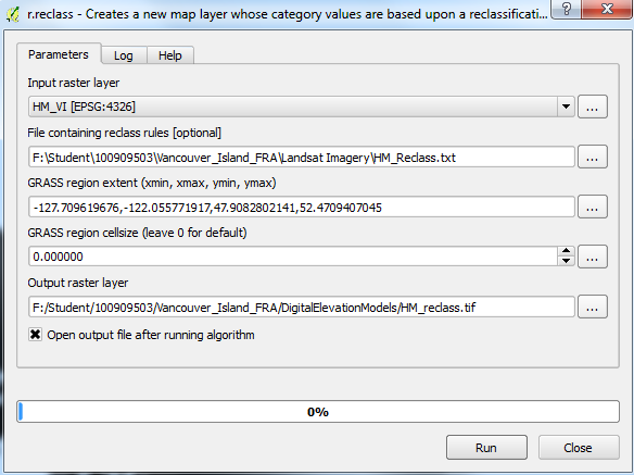
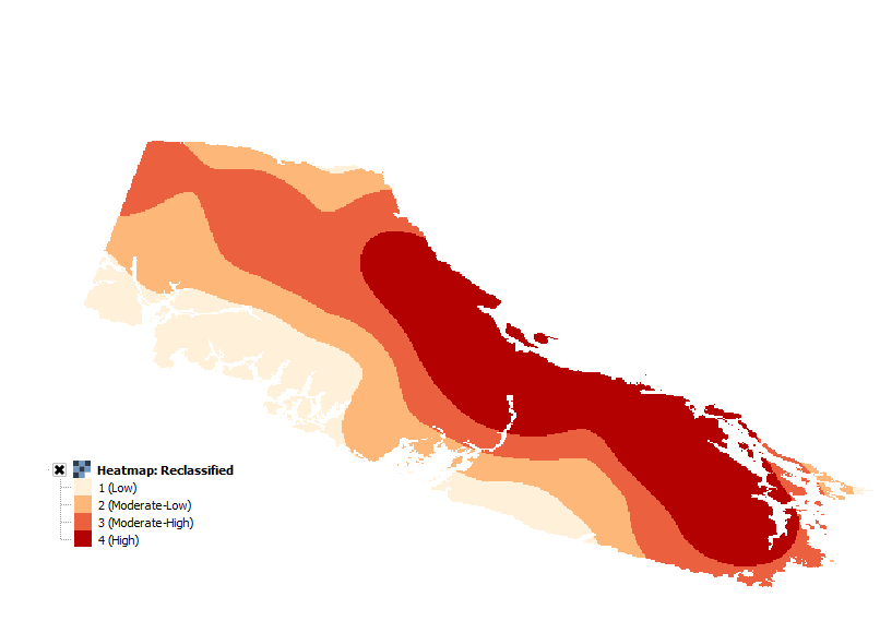
After you run the tool your heatmap based on the spatial pattern of points will apear as a raster and will have values associated with it - high values indicating areas where clustering is more present and low values indicating little to no clustering, you will want to use the clipper tool to clip it to the area of interest. The next step will be to reclassify the values of the heatmap outputted so you can calculate it later on. Use the r.reclass tool which is found in the advanced interface toolbox to complete it, after the heatmap is reclassified and the tool is run you will be able to use it in your calculation (Figure 22), open a word processor and type the following justification:

85 thru 125 = 4

50 thru 85 = 3

25 thru 50 = 2

0 thru 25 = 1

Figure 22. Clipping the heatmap raster to the study area, then reclassifying the heatmap long with the the output produced from reclassification.

Clipping, Buffering and Rasterizing Mitigation Factors

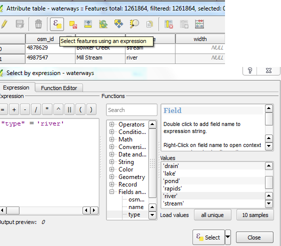
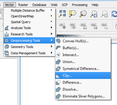
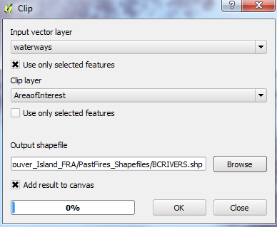
In this section we will be using the water polyline features downloaded from the Geofabrik, which is a server that enables a user to download up to date data derived from OpenStreetMap. We first looked under the attribute table of the file and felt that only rivers were to be selected for this analysis, to do so navigate to your waterways shapefile, right click your shapefile and open the Attribute Table and under Select by Attributes type the following justification: "type" = 'river' , you then will have all of rivers within British Columbia and then you will want to clip all of the selected features by the study are by navigating to the Vector tab and under the Geoprocessing tools, select the Clip tool and clip the input vector layer will be your waterways and ensure Use only selected features is checked on, while your clip layer will be your study area (Figure 23).

Figure 23. Select appropriate attributes, where to find the clip tool, along with the parameters in order to run the tool.

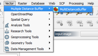
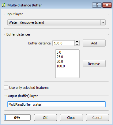
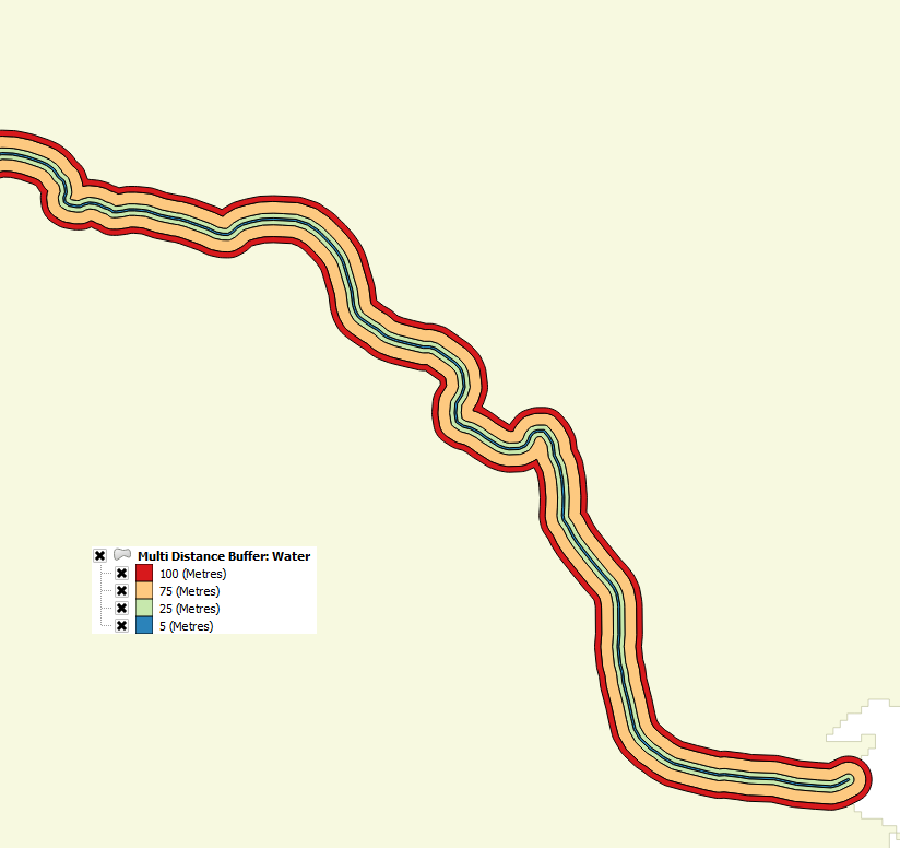
Since water is a mitigation factor for this analysis we will want to create a multi-ring buffer around the waterways, using the plugin we installed at the start of the tutorial open it up and input the newly clipped water bodies as the shapefile, and input appropriate buffer distances. For the purpose of our analysis we will use buffers at 5, 25, 50 and 100 metres (Figure 24).

Note: Your buffer shapefile may go over your study area, if this is the case you will need to use the Clip tool again, located under the Vector tab in Geoprocessing.

Figure 24. Where to find the multi-distance buffer tool, along with the appropriate parameters and the output of a single river feature.

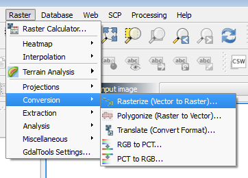
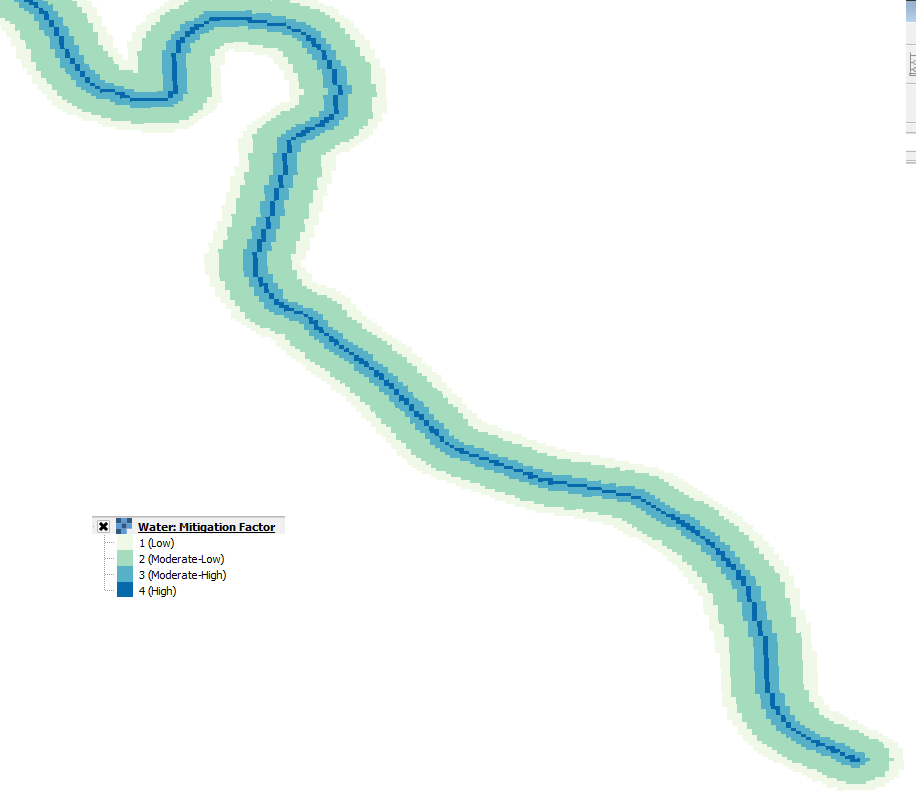
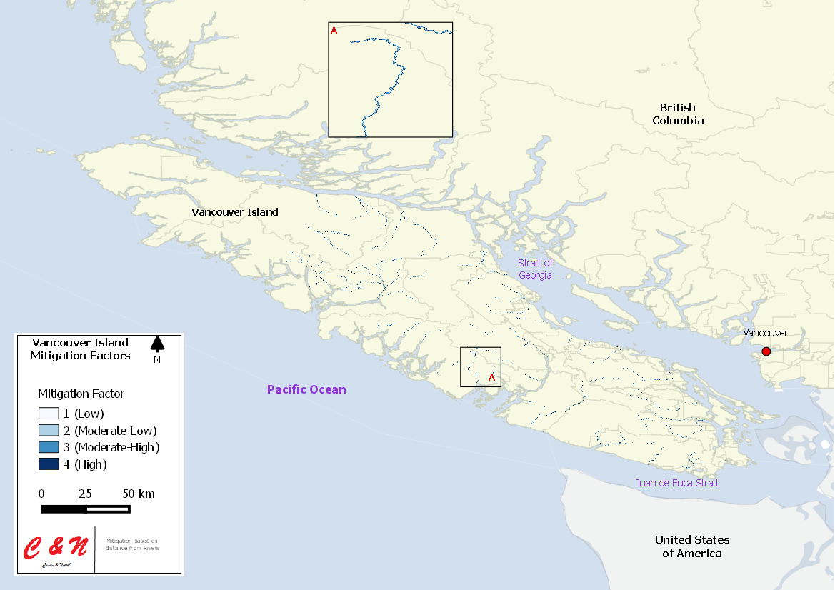
After you have run the tool, you will want to convert your newly created buffers into a raster, you will navigate to the Raster tab and under Conversion use the Rasterize tool in order to get your shapefiles into raster form, the conversion to raster will be based upon the values of the buffer created in the multi-distance buffer tool. After you have successfully converted the buffer shapefile into raster, you will want to reclassify the raster with the r.reclass tool found in the advanced interface toolbox, reclassification is based on the distances away from original polyline locations (Figure 25). The closer the buffer is to the original polyline the higher mitigation factor it plays thus a higher value is assigned to it, justification is as follows:

5 = 4

25 = 3

75 = 2

100 = 1

Figure 25. Where to find the rasterize tool, and the reclassified mitigation factor.

Spatial Joins, Identifying Areas of High Population and Vector Reclassification

In this section we will be using the Vancouver Island shapefile that we created using the select by features near the start of the tutorial, and will be joining the two in order to identify area of high population on the Island.

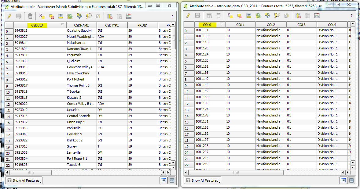
The first step is to open both Attribute tables by right clicking each dataset and clicking Open Attribute Table. Once you have done so, you can identify which have the same data in each attribute table, for our analysis the CSDUID from the Vancouver Island shapefile and COL0 from the population attribute data were the same (Figure 27), so we will create a spatial join based on this.

Figure 27. Attribute fields of both datasets that will be used in the join.

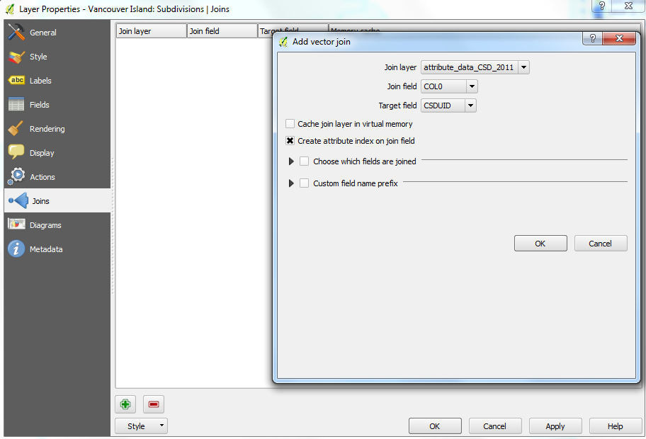
The next step will be to Right click your Vancouver Island shapefile, open Properties and on the left side of Layer Properties you will see a tab called Joins.

It will open a prompt and ask you which Join Layer (Population attribute data) you would like along with Join Field (COL0) and the Target Field (CSDUID) which we all identified in the last step, ensure Create attribute index on join field is also selected (Figure 28).

Figure 28. How to add a vector join to obtain population data per CSD.

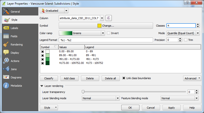
Your Vancouver Island shapefile will also now have the population data, which will be under the header named COL7, you can change the symbology to your desire, it is a good idea to do so because it will help with the reclassification method. So again open your Layer Properties naviagate to the Style tab, using COL7 a Quantile mode with 4 classes and apply whichever color ramp you wish to the data (Figure 29).

Figure 29. The style tab of layer properties, which was used in order to visualize areas of high population on the Island.

Since your shapefile is not permanent you will have to save it as a new shapefile, by right clicking it and saving at as a new shapefile, use the Clip tool located under the Vector and Geoprocessing tabs and clip the new shapefile to the study area.

The next step will be to create a raster using the Rasterize tool, found in the Raster tab, use COL7 data as the way to create a raster, then reclassify based on the Quantile classification use the r.reclass tool to do so, use the following rule;

0 thru 88 = 1

88 thru 491 = 2

491 thru 4283 = 3

4283 thru 109752 = 4

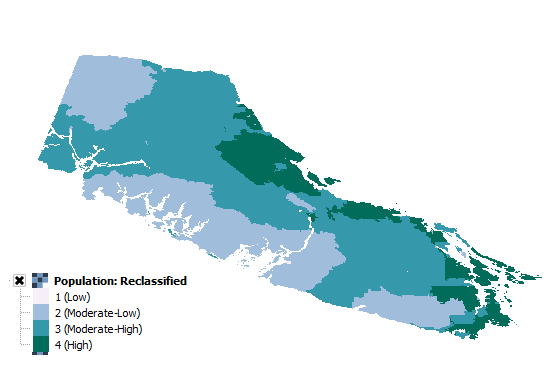
After the tool has run you should have your new raster ready for the vulnerability calculations (Figure 30).

Hazard, Vulnerability and Mitigation Raster Calculations

In this section we will be using the Raster Calculator in order to create hazard, vulnerability and mitigation maps, the three categories that were decided upon in the #Introduction.

Hazard Calculation

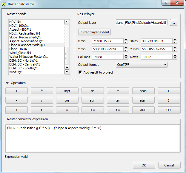
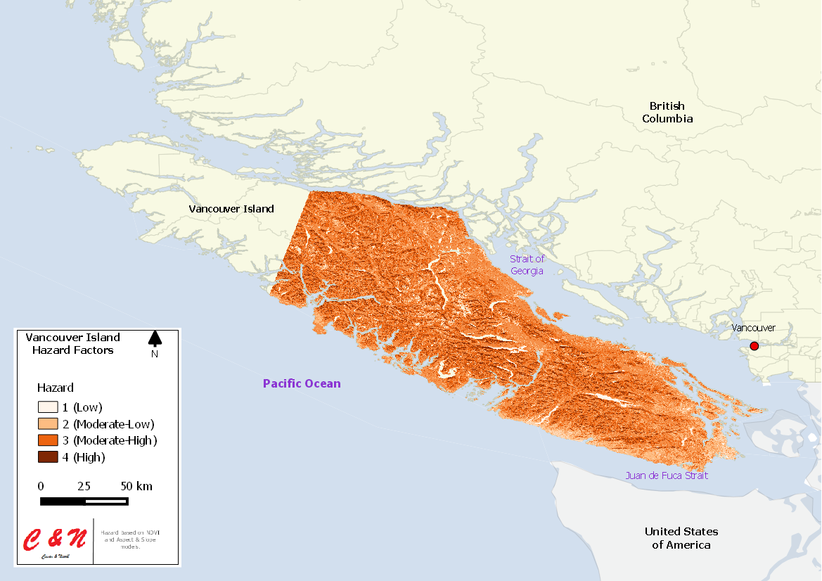
The hazard calculation will take into account the NDVI and slope & aspect rasters that were created, we decided that they equally play important roles in a forest fire thus deciding to weight them equally. The following weight was used in the calculation, NDVI - 50% + Slope & Aspect - 50%.

To complete this calculation in QGIS, open the Raster Calculator, double click your NDVI and Slope & Aspect rasters, and type the following equation:

(0.5 * NDVI) + (0.5 * Slope & Aspect)

This will create your final hazard map taking into account both factors, maximum value will remain 4 and minimum will remain 1.

Vulnerability Calculation

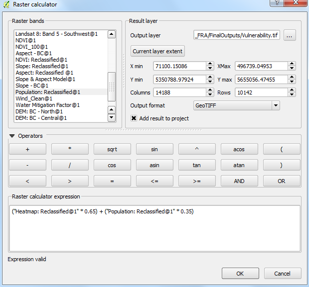
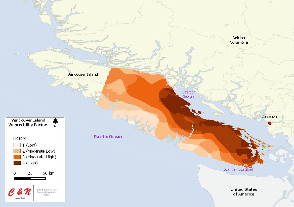
The vulnerability calculation will take into account the heatmap (past fires) and population density, we decided that the location of past fires has a higher vulnerability weight than population density per tract. The following weight was used in the calculation, Heatmap (Past Fires) - 65% + Population - 35%.

To complete this calculation in QGIS, open the Raster Calculator double click your heatmap raster and population rasters, and type the following equation:

(0.65 * heatmap) + (0.35 * population density)

This will create your final vulnerability map taking into account both factors, maximum value will remain 4 and minimum will remain 1.

Mitigation Calculation

Since the water raster is the only mitigation factor there will be no need for calculation, and the raster created can be used in the final calculation.

Final Weighted Calculation using Raster Calculator

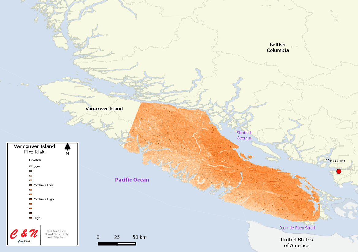
In this section we will be calculating the overall risk the study area has based on all of the factors identified in previous sections. Using the maps we just produced from the hazard, vulnerability and mitigation section, we will again use the Raster Calculator to complete the weighted calculation. Hazard and vulnerability will be added together, while the mitigation is subtracted from the two. Hazard is given a weight of 60%, while vulnerability is given a weight of 30% and finally, mitigation is given a weight of 10%.

Open the Raster Calculator and type the following equation, and run the tool: (0.6 * hazard) + (0.3 * vulnerability) - (0.1 * mitigation)

After the tool has run, you will have your final Risk output combining all of the factors together.

Identifying Zones of High Risk Using Zonal Statistics

To identify zones in order to make it easier for planning against risk, we created 25 kilomtere by 25 kilometre vector grids, and ran zonal statistcs to understand the zones of high risk.

To do so you must first create a polygon grid, navigate to Vector tab and under Research Tools, you will find the tool named Vector Grid. Create the appropriate grid size for your analysis, we chose 25km by 25km. Then navigate to the advanced toolbox interface and type in Zonal Statistics, click the QGIS Zonal Statistics tool and run it on the final map you created with relationship to the grid. After that has run, you can open up your attribute table and take a look at the 'mean' value outputed from the tool, and change the symbology of the grid based upon this.

Conclusion

In conclusion we ran some tools did some cool things and had a great time