Supervised classification in QGIS

Purpose

Every day thousands of satellite images are taken. To work with these images they need to be processed, e.g. they need to be classified. Since Remote Sensing software can be very expensive this tutorial should provide an open-source alternative: the Semi-automatic-classification plugin (SCP) in QGIS. You can already find a tutorial about the SCP here [1]. With this tutorial you can extend your ability to use the SCP while running through a supervised land-cover classification.

Introduction

Land-cover classification classifies every pixel to a defined class using the spectral signatures. To define the classes region of interests (ROI) must be set.

Installing the Software and SCP

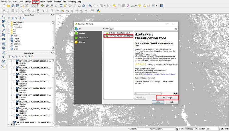
To start the tutorial you have to download the latest version of QGIS which is QGIS 3.4.1. "Bonn" and can be found here[2]. Make sure to download the proper version for your PC (34bit vs. 64bit). After installing the software the the Semi-automatic classification Plugin must be installed into QGIS. Navigate to the menu at the top to Plugin and select Manage and Install Plugins. Following the picture, the SCP can be found while typing "semi" in the search bar. Click install plugin and now you should be able to see the SCP Dock at the right or left side of your user surface.

Obtaining the Data

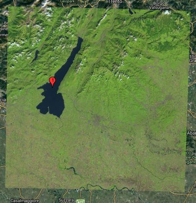
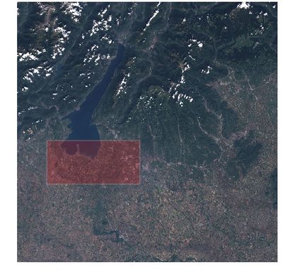
In this Tutorial, Sentinel-2 Data from the south of Lake Garda, Italy is used to run the classification. The data can be downloaded from the USGS Earth Explorer website here[3]. You can found a explanation how to download data from the Earth Explorer in the Tutorial Remote Sensing Analysis in QGIS. To find the same picture as used in this tutorial search for Lake Garda and select the time period from August to October 2018. Among Data Sets select Sentinel-2 and you should find the following picture:

It has the ID L1C_T32TPR_A008056_20180921T101647 and is shot the 21st of September 2018.

Unpack the Data

The downloaded data is packed in a zip-File. Therefore, you have to unzip the Data before working with it. Afterwards you can find the image data under GRANULE → L1C_T32TPR_A008056_20180921T101647 → IMG_DATA. Here you can find for each band of the Sentinel satellite a separate JPEG file.

Preprocessing Data

Load the Data into QGIS

To load the Data into QGIS navigate to Layer at the top your user surface. Choose Add Layer, and then Add Raster Layer.... You should see the Data Source Manager now. Leave "File" selected like it is in default. Under Datasets you can navigate to the directory described above. Make sure to load all JPEG files into QGIS except the file of band 10: T32TPR_20180921T101019_B10.

Creating an Band set

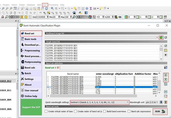
The next step is to create a band set. For this approach navigate to the SCP button at the top of the user surface and select Band set. Under Multiband image list you can load the images into SCP and then into the Band Set 1. Make sure the layers are in the right order and select Sentinel-2 under Quick wavelength units. The picture below should help to understand these steps.

Clip the Data

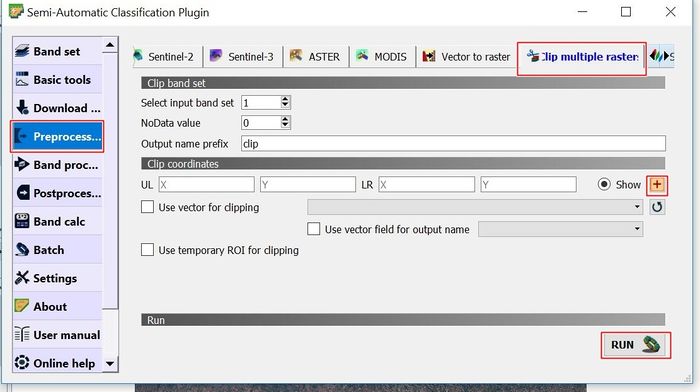
For a basic classification the area covered by the picture is very big. Therefore, we can clip the data and only work with a part of the picture. Navigate to the SCP button at the top of the user surface, under Preprocessing you find clip multiple Raster. Your surface should look similar like in the picture below. Leave the number 1 at band set as we have defined it in the previous step.

To clip the data press the orange button with the plus. Minimize the SCP window and you can now define the area you want to work with while clicking with the right button on your mouse. I suggest to define an area south of the mountains to avoid dealing with mountain shadows in the classification. In addition in the south of the pictures there are no clouds. For instance, like this:

After defining the section under coordinate there should occur be numbers. Click run and define an output folder.