Difference between revisions of "Flood Risk Assessment using Grass GIS"
Rjmitchell (talk | contribs) |
Rjmitchell (talk | contribs) |
||
| Line 38: | Line 38: | ||
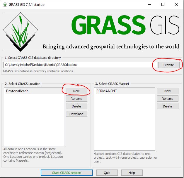
: 3. Create a '''New Location''' for your workspace in Step 2 |
: 3. Create a '''New Location''' for your workspace in Step 2 |
||
: 4. Specify the Project Location and Location Title, select '''Next''' |
: 4. Specify the Project Location and Location Title, select '''Next''' |
||
[[File:Startup.PNG]] |
|||
: 5. Select the default ''Select EPSG code of spatial reference system'' and click on '''Next''' |
: 5. Select the default ''Select EPSG code of spatial reference system'' and click on '''Next''' |
||
: 6. Search for ''NAD83 / Florida East'', or input the EPSG code 26958 and click on '''Next''' |
: 6. Search for ''NAD83 / Florida East'', or input the EPSG code 26958 and click on '''Next''' |
||
| Line 74: | Line 75: | ||
: 2. Input this expression to simulate water levels of 6m: DaytonaFLOOD2m = '''( ( DaytonaSRTM@PERMANENT <= 6 ) == 1 ) & ( ( DaytonaSRTM@PERMANENT >= 6 ) == 0 ) *supplement DaytonaSRTM with whatever you named the ''SRTM DEM'' file* |
: 2. Input this expression to simulate water levels of 6m: DaytonaFLOOD2m = '''( ( DaytonaSRTM@PERMANENT <= 6 ) == 1 ) & ( ( DaytonaSRTM@PERMANENT >= 6 ) == 0 ) *supplement DaytonaSRTM with whatever you named the ''SRTM DEM'' file* |
||
: 3. Click on '''Run''', make sure the ''Add created raster map into layer tree'' option is selected before doing so |
: 3. Click on '''Run''', make sure the ''Add created raster map into layer tree'' option is selected before doing so |
||
[[File:Flood2m. |
[[File:Flood2m.PNG]] |
||
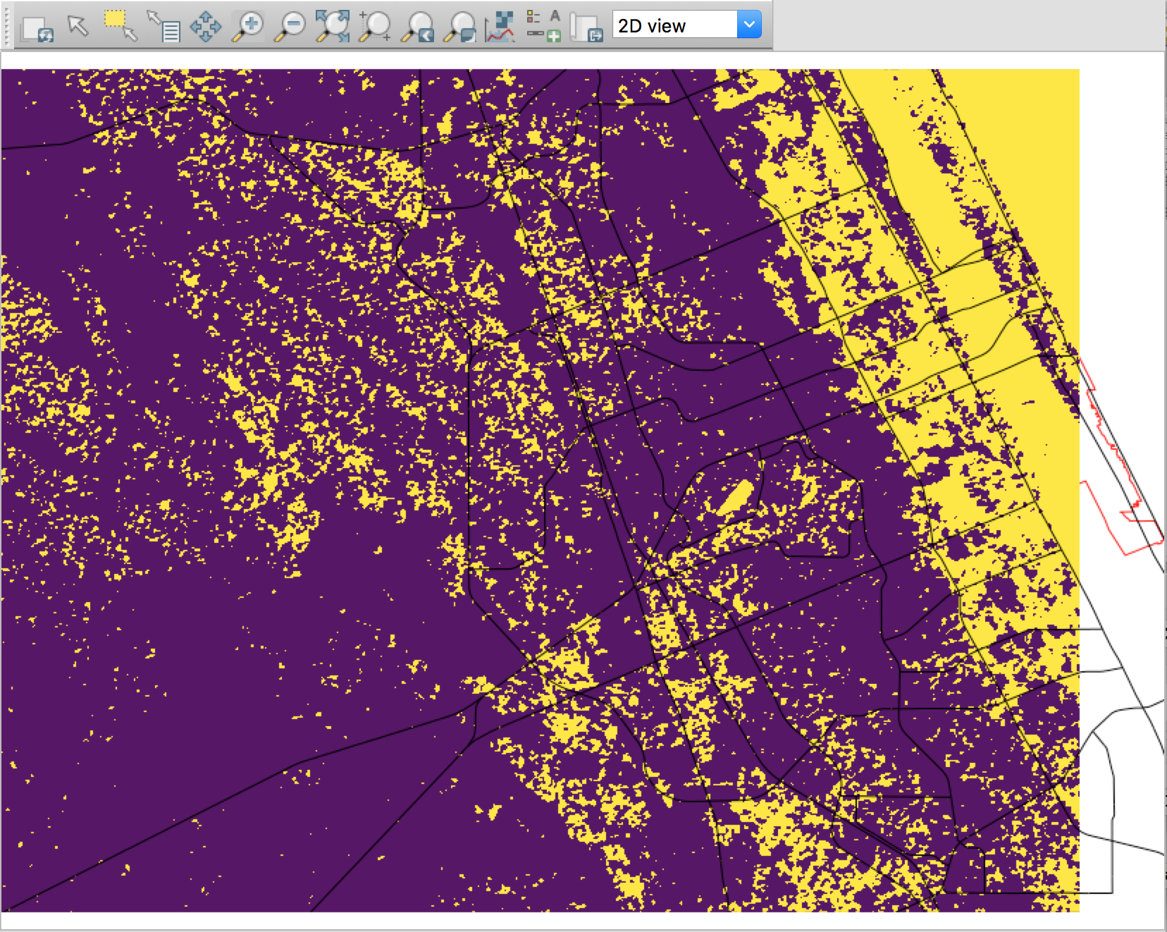
The resultant raster map shows which areas are inundated (yellow) and the non-inundated areas (purple) at 2m sea level rise. Next we will create another raster map showing an example of 5m of rising sea level. |
The resultant raster map shows which areas are inundated (yellow) and the non-inundated areas (purple) at 2m sea level rise. Next we will create another raster map showing an example of 5m of rising sea level. |
||
Revision as of 19:02, 21 December 2018
Contents
Introduction
With global climate change becoming the prevalent issue of the generation, more and more people are using GIS to emulate the effects of climate change in their communities. Rising water levels are especially of concern as humans tend to settle near water bodies and coastal areas. This tutorial aims to give an introductory lesson into conducting a very basic flood risk assessment using open source software and data. This tutorial utilizes Grass GIS and data from the city of Daytona Beach, FL, USA, a popular vacation destination on the Atlantic Coast.
Software and Data
This tutorial uses the latest version of Grass GIS 7.4.1, which can be downloaded for Windows, MacOSX, and Linux from their website ([1]). Once installed, we can focus on collecting the data needed. GRASS GIS can be operated with script, but this tutorial was developed for the amateur user and will not focus on Python script application.
The data used for this lesson is derived from two main sources, the US Geological Survey Earth Explorer tool ([2]) and the City of Daytona Beach website ([3]), both are open source, although the USGS requires you to create an account to access their data.
First, let's begin by collecting the data needed from the City of Daytona Beach:
- 1. Open the link provided from above
- 2. Scroll down and select the Boundaries icon
- 3. There are several scales to choose from, select the Daytona Beach Boundary file
- 4. Select Download from below the bottom-right corner of the image, and download as a shapefile
- 5. Extract data to appropriate folder
- 6: Return to the main menu and select the Transportation icon
- 7. Select the Major Roads file
- 8. Select Download from below the bottom-right corner of the image, and download as a shapefile
- 9. Extract data to appropriate folder
Next, we will collect the data from the USGS website:
- 1. Open the link provided from above
- 2. Select the Data Sets tab at the top of the window
- 3. Expand the Digital Elevation menu, expand the SRTM submenu, select SRTM 1 Arc-Second Global
- 4. Return to the Search Criteria tab
- 5. Type Daytona Beach into the Address/Place field and click on Show
- 6. Select the Daytona Beach, FL, USA file and click on Results
- 7. Click on the Show Metadata and Browse
- 8. Click on Open New Window
- 9. Select Download, you will need to login with your account at this point if you haven't already, download as TIFF
- 10. Extra data to appropriate folder
Methods
Starting a GRASS session
Now that we have our data collected, we can open Grass GIS and setup the tutorial session:
- 1. Open Grass GIS
- 2. Browse to your selected directory in Step 1
- 3. Create a New Location for your workspace in Step 2
- 4. Specify the Project Location and Location Title, select Next
- 5. Select the default Select EPSG code of spatial reference system and click on Next
- 6. Search for NAD83 / Florida East, or input the EPSG code 26958 and click on Next
- 7. Select datum 2 for Used in Florida and click on OK
- 8. Click on Finish
- 9. Select your new Location and click on Start GRASS Session
Importing Vector Data into GRASS
The GRASS session is now setup, and we can start importing the data we collected from earlier, starting with the boundary file
- 1. Under the File tab from the top of the window, select Import Vector Data and choose the Import of common vector formats [v.in.ogr]
- 2. Browse to the location of the Daytona Beach boundary file
- 3. Under the Optional tab, select the Override projection check and click on Run
- 4. At the top toolbar select the Add vector map layer button
- 5. Select the boundary file under the drop-down menu and click OK
- 6. Right-click on the boundary file in the Layer Manager and select Set computational region from selected map(s), this creates an area of interest (AOI) and sets the computational extent around the city
Next, we will import the major roads file using the same process as above, without setting the computational region (Step 6)
Importing Raster Data into GRASS
Now we can import the SRTM DEM we downloaded earlier from the USGS:
- 1. Under the File tab, select Import raster data and choose Import of common raster formats [r.in.gdal]
- 2. Browse to the location of the SRTM DEM and input a name for the output raster map
- 3. Select Override projection check under the Projection tab and click on Run
Changing Symbology
Now that we have the data displayed, we can adjust the symbology to better suit our applications:
- 1. Right-click on the SRTM DEM layer and select Set color table
- 2. Ensure that the correct raster file is selected
- 3. Under the Define tab, click on the drop-down menu under Name of color table and select the elevation color table, and click on Run
- 4. Right-click on the boundary file and select Properties
- 5. Under the Colors tab, select a color for the boundary itself and check Transparent for the Area fill color, and click on OK
Creating flooding scenarios
We have our map ready to run a basic flood risk assessment using the raster calculator. The lowest points of elevation in Daytona Beach is approximately 4m, but we will simulate an initial rise of 2m to conservatively determine the effects of flooding.
- 1. Under the Raster tab, select Raster map calculator [r.mapcalc]
- 2. Input this expression to simulate water levels of 6m: DaytonaFLOOD2m = ( ( DaytonaSRTM@PERMANENT <= 6 ) == 1 ) & ( ( DaytonaSRTM@PERMANENT >= 6 ) == 0 ) *supplement DaytonaSRTM with whatever you named the SRTM DEM file*
- 3. Click on Run, make sure the Add created raster map into layer tree option is selected before doing so
The resultant raster map shows which areas are inundated (yellow) and the non-inundated areas (purple) at 2m sea level rise. Next we will create another raster map showing an example of 5m of rising sea level.
- 1. Under the Raster tab, select Raster map calculator [r.mapcalc]
- 2. Input this expression to simulate water levels of 6m: DaytonaFLOOD2m = ( ( DaytonaSRTM@PERMANENT <= 9 ) == 1 ) & ( ( DaytonaSRTM@PERMANENT >= 9 ) == 0 ) *supplement DaytonaSRTM with whatever you named the SRTM DEM file*
- 3. Click on Run, make sure the Add created raster map into layer tree option is selected before doing so
Results
By toggling between the original SRTM DEM, 2m Flooding, and 5m Flooding layers, we can ascertain the levels of flooding we could see in areas in and around Daytona Beach.

