Geomorphometric Analysis using Whitebox Tool

Purpose

The purpose of this tutorial is to provide a clear and practical introduction to conducting a full geomorphometric analysis using WhiteboxTools within QGIS. This guide is designed for students, researchers, geoscientists, environmental analysts, and anyone working with terrain data. By following the step-by-step workflow, users will learn how to preprocess a DEM, extract primary and secondary terrain attributes, and visualize landforms using free, open-source tools. The resulting geomorphometric products can enhance understanding of the topography, structure, and processes shaping a study area, and are suitable for use in academic reports, research publications, and applied geospatial projects

Introduction

What is the geomorphometric

Geomorphometry is the science of quantitatively measuring and analyzing the physical features of the Earth’s surface. It focuses on extracting numerical parameters—such as slope, aspect, curvature, roughness, and landform indices—from Digital Elevation Models (DEMs). The goal is to describe terrain in a mathematically precise way, allowing researchers to model processes, compare landscapes objectively, and automate landform classification. In geomorphometry, every element of the terrain is expressed using measurable values, for example the slope expressed in degrees or percent rise, curvature expressed as concave or convex values, or drainage indices extracted using computational algorithms.

Advantages of Geomorphometric Analysis

Conducting a geomorphometric analysis offers major advantages for geomatics, environmental as well as geosciences research. It transforms raw elevation data into quantifiable, reproducible metrics, enabling precise terrain interpretation that is impossible through visual observation alone. These quantitative outputs support a wide range of applications, including hydrological modeling, erosion assessment, landform classification, hazard mapping, suitability analysis, and machine-learning workflows. Because geomorphometric variables are standardized and scalable, they allow researchers and students to analyze landscapes efficiently, compare regions objectively, and produce high-quality results suitable for scientific publications or decision-making.

Advantage of Whitebox Tool for geomorphometric analysis

WhiteBox tool offers several significant advantages for performing geomorphometric analysis, particularly in an academic or research environment. As a free and open-source GIS processing library, it provides access to a wide range of terrain-analysis algorithms without the cost barriers associated with commercial software. WhiteboxTools is optimized for raster processing and uses efficient parallel computation, allowing users to work with large DEMs and complex workflows quickly and reliably. Its seamless integration with QGIS makes it easy for students and researchers to incorporate advanced geomorphometric tools into everyday GIS projects.

Another major advantage is the availability of specialized geomorphometry functions (such as curvature, ruggedness, topographic position, downslope indices, and feature-preserving smoothing) that are not always included in standard GIS packages. These tools help users extract meaningful quantitative metrics describing the shape and structure of the landscape. Because WhiteboxTools is actively maintained and scientifically oriented, it is ideal for teaching, research, hydrology, geomorphology, environmental modeling, and preparing high-quality outputs suitable for academic reports and publications.

Target audience and scope

This tutorial is designed for anyone interested in understanding and applying geomorphometric analysis to quantify and interpret landscape morphology. It provides a step-by-step methodology to extract meaningful geomorphometric parameters from a Digital Elevation Model (DEM) using free and open-source software, specifically WhiteboxTools integrated within QGIS. The workflow begins with plugin installation and data acquisition, followed by DEM preprocessing and noise reduction, and then guides the user through the computation and interpretation of key morphometric parameters such as slope, curvature, directional relief, and topographic indices.

Because of its progressive and structured approach, this tutorial is suitable for students at the undergraduate and graduate levels, as well as professionals and researchers seeking an introduction or practical refresher in geomorphometry. While the methodology can be applied across many disciplines, it is particularly relevant for geomatics specialists, geographers, geologists, environmental scientists, and hydrologists, as well as anyone working with terrain analysis, landform classification, or landscape modeling

Getting started

Plugin installation

To install the WhiteboxTools plugin in QGIS, the process begins by opening the Plugins menu and selecting Manage and Install Plugins. In the search bar, typing “Whitebox” displays the list of available Whitebox-related extensions. The correct plugin to install is WhiteboxTools for QGIS. If the plugin does not appear automatically, the standalone WhiteboxTools package must be downloaded from the official website: https://www.whiteboxgeo.com/download-whiteboxtools . After downloading, the folder containing the executable file ( whitebox_tools.exe ) should be extracted. Once installed, the path to the executable must be configured in QGIS: this is done by navigating to Settings → Options → Processing → Providers → WhiteboxTools, and selecting the extracted whitebox_tools.exe file as the executable (fig 1). After this configuration is completed, the full suite of geomorphometric tools becomes available in the QGIS Processing Toolbox under WhiteboxTools

Figure 1: WhiteboxTools Plugin Setup in QGIS

Data acquisition

For this tutorial, the elevation data are obtained from the Shuttle Radar Topography Mission (SRTM) using the USGS EarthExplorer portal. SRTM provides freely available digital elevation models at 1-arc-second (~30 m) resolution, which is sufficient for regional-scale geomorphometric analysis. The selected SRTM tile(s) covering the study area are downloaded from EarthExplorer, unzipped, and stored in the project workspace so they can be imported into QGIS and processed with WhiteboxTools.

Step-by-step: Downloading SRTM from EarthExplorer

Open the USGS EarthExplore website and Sign in with a USGS account (or create a free account if necessary) using the Login button in the top-right corner. In the Search Criteria tab, define the area of interest: Use the map to zoom to the study area and click Use Map; or enter coordinates or place names under Address/Place; or specify a polygon/rectangle using the Coordinate tools.

Set an appropriate Date Range (for SRTM, the default historical range is generally acceptable). Switch to the Data Sets tab and expand Digital Elevation → select SRTM → SRTM 1 Arc-Second Global. Click Results at the bottom of the interface. The list of available tiles for the defined area appears. In the results list, identify the tile(s) covering the study area and click the Download icon (downward arrow) for each. In the download options, choose the GeoTIFF (or equivalent DEM) format. Once the download is complete, extract the contents of the ZIP archive(s) into a dedicated project folder.

Fundamental Knowledge

Geomorphometric parameters derived using WhiteboxTools are computed from a Digital Elevation Model (DEM). For many tools, the Z conversion factor is an optional parameter. This factor is required only when the vertical and horizontal units of the DEM are different. This situation occurs when elevation values (Z) are expressed in one unit (for example, feet), while the spatial reference system of the DEM is expressed in another unit (such as meters or geographic coordinates in degrees).

This mismatch is common when using LiDAR-derived DEMs from the USGS, where elevation is often stored in feet while the horizontal projection is in meters. If geomorphometric derivatives are computed without applying the appropriate Z conversion factor under these conditions, the results will be geometrically inconsistent and physically incorrect.

For example, when elevation is in feet and horizontal units are in meters, the Z conversion factor must be set to 0.3048, since 1 foot = 0.3048 meters. Applying this correction ensures accurate slope, curvature, and terrain derivative calculations.

Another good thing to know is that geomorphometric parameters are scale-dependent. Window size, search distance, and filter dimensions directly influence the spatial patterns detected. Smaller windows highlight local micro-topography, while larger windows emphasize broader landforms. Parameter values used in this tutorial were selected to balance local detail and regional context

DEM Smoothing

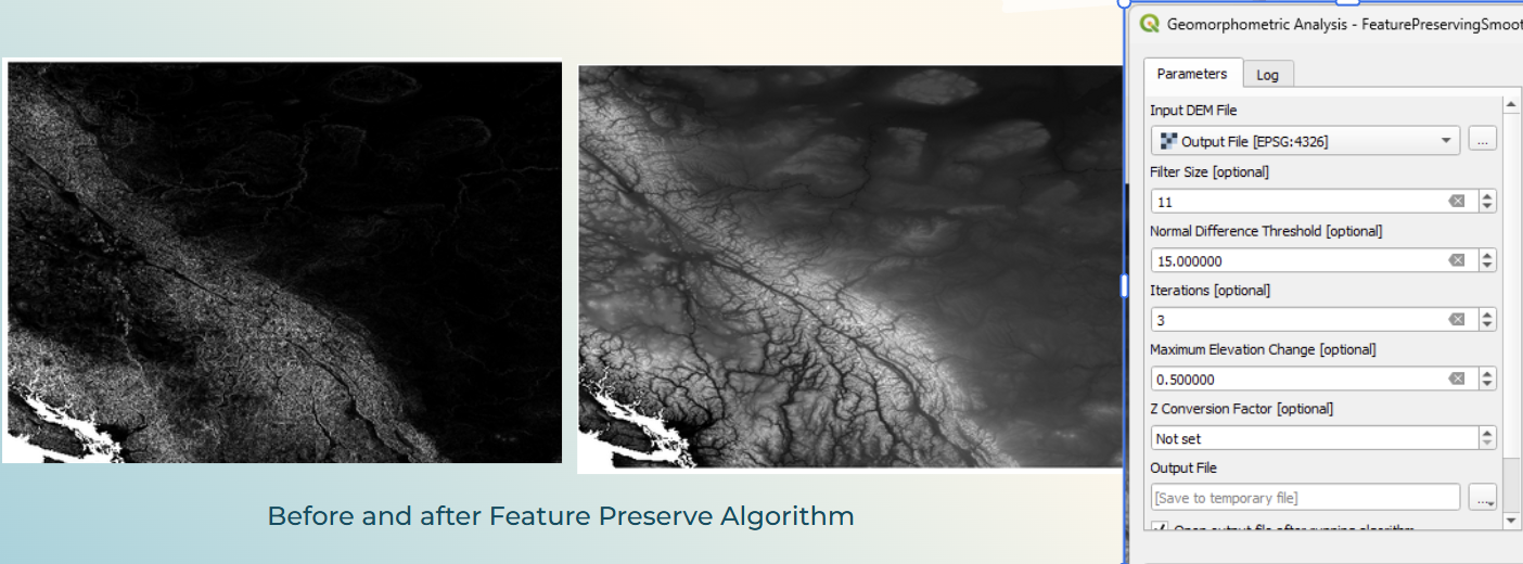
When working with a Digital Elevation Model (DEM), it is important to keep in mind that many elevation datasets were created several years ago. As a result, it is common to encounter DEMs that contain noise, interpolation artifacts, or small irregularities caused by data acquisition and processing methods. In such cases, the Feature Preserving Smoothing tool available in the WhiteboxTools geomorphometric package can be used to reduce noise and enhance the visibility of true terrain features. This algorithm works by first calculating the 3D surface normal vectors for each grid cell based on a 3×3 neighborhood. The normal vector field is then smoothed by giving more weight to neighboring cells with similar orientation (lower angular difference), and the elevation values are updated using the smoothed normal vectors. This process effectively removes high-frequency noise while preserving important geomorphological structures such as ridges, valleys, and slope breaks.

To properly configure this tool, the key parameters to consider are the filter size, the normal difference threshold, and the number of iterations. Increasing the normal difference threshold increases the level of smoothing, because more neighboring values are included in the filtering process, generally resulting in a smoother surface.

Figure 2: DEM denoising

The default filter size of 11 works well in many cases and provides a good balance between noise reduction and feature preservation. The Feature Preserving Smoothing tool can be accessed in QGIS by navigating through WhiteboxTools → Geomorphometric Analysis → FeaturePreservingSmoothing.

Topographic visualization

Hypsometrically Tinted Hillshade

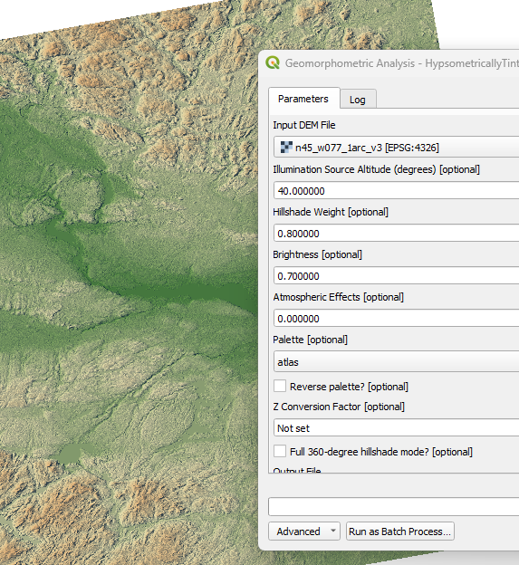
The Hypsometrically Tinted Hillshade is a visualization technique that combines a traditional hillshade with a colored Digital Elevation Model (DEM) to enhance terrain interpretation. Also called Swiss-style hillshade, this method integrates multiple illumination directions with elevation-based color gradients to produce a visually intuitive and informative representation of the landscape. This tool is particularly important in geomorphometric analysis because it allows users to easily identify major landforms such as ridges, valleys, plateaus, and escarpments, while maintaining a realistic sense of terrain structure.

To generate this output, go to WhiteboxTools → Geomorphometric Analysis → Hypsometrically Tinted Hillshade. This tool includes several important parameters that control the final visualization. The illumination altitude parameter defines the height of the virtual light source and influences how shadows are cast across the terrain surface. The hillshade weight controls the balance between the hillshade and the elevation color ramp: higher values emphasize relief and terrain texture, while lower values place more emphasis on elevation differences through color. The brightness option enhances overall contrast, improving the visibility of subtle geomorphic features. Together, these parameters allow the user to produce a clear, visually appealing map that supports both qualitative terrain interpretation and high-quality cartographic presentation.

Figure 2: Hypsometrically tinted Hillshade generated with Whitebox Tools

Hillshade

Hillshade is a black and white visualization of a Digital Elevation Model (DEM) that simulates how the terrain would appear if illuminated by a light source, typically representing the sun. It is computed using a specified azimuth (the horizontal direction of illumination, from 0° to 360°) and altitude (the vertical angle of the light source above the horizon). By modeling the interaction between light and topography, hillshade enhances the visual perception of relief, making variations in elevation, slope, ridges, valleys, and other landforms easier to identify.

Hillshade is a fundamental tool in geomorphometric analysis because it does not modify the DEM values, but instead improves terrain interpretation and visualization. It is particularly useful for identifying subtle landforms, drainage patterns, slope breaks, and structural lineaments that may not be immediately visible in raw elevation data. For best results, the azimuth should be chosen to illuminate the dominant terrain orientation of the area of interest, as certain landforms may appear more clearly when lit from specific directions. The altitude parameter controls the height of the light source; lower values emphasize shadows and relief, while higher values produce a smoother appearance. The Z conversion factor is optional and should only be applied when the vertical and horizontal units of the DEM differ.

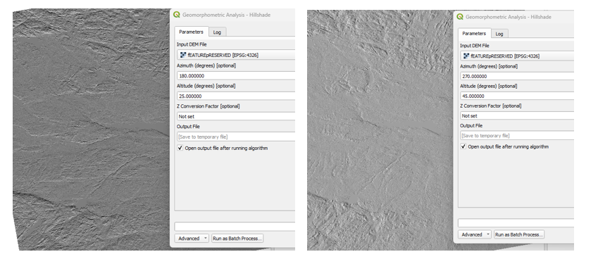
To compute a hillshade in QGIS using WhiteboxTools, open the Whitebox Tools interface, navigate to Geomorphometric Analysis, and select Hillshade. Specify the input DEM, set the azimuth and altitude parameters according to the study area, adjust the Z conversion factor if required, and then run the tool to generate the hillshade raster.

In the left image Figure4_hillshade, using an azimuth of 180° and an altitude of 25°, valley networks and linear depressions are strongly emphasized, making drainage patterns more apparent. In contrast, the right image, generated with an azimuth of 270° and an altitude of 45°, highlights convex landforms such as ridges and slope crests more clearly. By adjusting the azimuth and altitude values, users can selectively enhance different geomorphological features. Experimenting with these parameters allows for a better interpretation of terrain structure, improves landform recognition, and supports more accurate geomorphometric analysis.

Figure 3: Comparison of Hillshade Rendering Using Different Illumination Parameters

Contours (To add)

Contours are one of the most classical and widely used representations of topography. A contour line connects points of equal elevation on a surface, allowing the three-dimensional shape of the terrain to be visualized on a two-dimensional map. The spacing between contour lines provides direct information about slope: closely spaced contours indicate steep terrain, while widely spaced contours represent gentle or flat areas. In geomorphometric analysis, contours are particularly useful for identifying ridges, valleys, depressions, drainage patterns, and breaks in slope, and they also serve as a visual validation tool for the quality of the DEM.

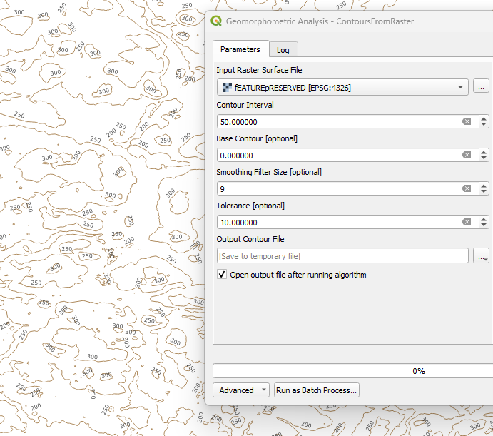
In WhiteboxTools, contours are generated directly from a raster surface such as a DEM. The most important parameter is the contour interval, which defines the vertical distance between successive contour lines. Smaller intervals produce more detailed contour maps but can lead to clutter in rugged terrain, while larger intervals emphasize regional topographic trends. Optional smoothing can be applied to reduce angular artifacts inherited from raster resolution, producing more cartographically pleasing contours. Contours remain an essential complement to shaded relief and slope maps, especially for interpretation, mapping, and communication of terrain structure.

To generate contours in QGIS using WhiteboxTools, navigate to WhiteboxTools → Geomorphometric Analysis → ContoursFromRaster, select the DEM, define an appropriate contour interval, and run the tool.

Figure 5. Contour Lines Derived from the DEM Using WhiteboxTools

Local geomorphometric parameter

Slope

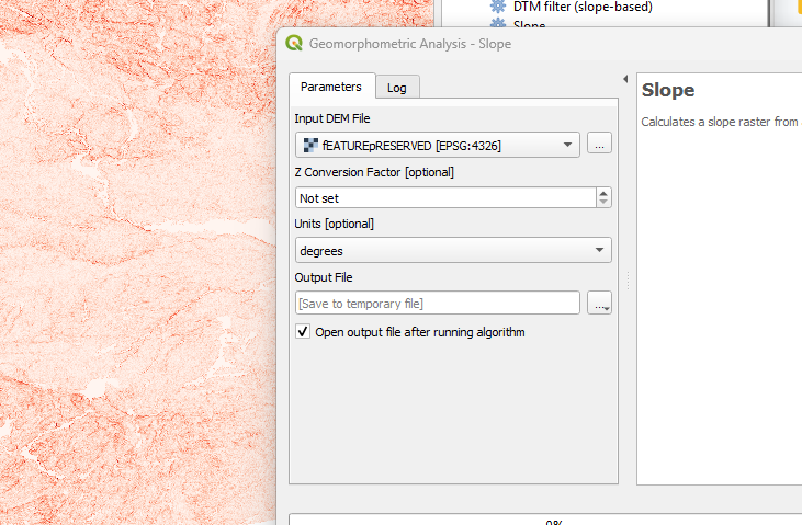
The slope describes how the terrain elevation varies across the landscape. It is expressed in degrees, radians, or percentage and represents the rate of maximum elevation change at each cell of a Digital Elevation Model (DEM). Slope is one of the most fundamental geomorphometric parameters because it directly controls many geomorphic and environmental processes. Steeper slopes generally experience greater erosion, faster surface runoff, and lower soil moisture, while flatter areas favor sediment accumulation and more stable landforms. Slope is also essential for identifying ridges, valley sides, plateaus, and areas prone to landslides or rapid hydrological flow.

To compute the slope in QGIS, open the WhiteboxTools plugin and navigate to Geomorphometric Analysis → Slope. The main input parameter is the DEM. The Z conversion factor must be applied only if the vertical and horizontal units of the DEM are different. The output type can be set to degrees (most commonly used), radians, or percent slope, depending on the application. These parameters ensure accurate and meaningful slope computation for geomorphometric analysis

Figure 4: Slope Map Derived from the Feature-Preserved DEM

.

Curvature

Curvature describes the local shape and orientation of a land surface and is a key quantity in geomorphometry. Using concepts from differential geometry, surface curvature provides a rigorous mathematical description of whether the terrain at a given point is convex, concave, or flat, based on the second derivative of elevation. In grid-based analysis, curvature is computed cell by cell by fitting a surface through each cell and its eight neighbors. Different curvature components capture different aspects of terrain form: profile curvature is measured in the direction of maximum slope and influences flow acceleration or deceleration along the slope, while plan curvature is measured perpendicular to the slope direction and affects the convergence or divergence of flow across the slope. Positive curvature values typically indicate convex surfaces (e.g., crests and spurs), negative values indicate concave surfaces (e.g., hollows and channels), and values near zero indicate planar surfaces. Because these patterns control water flow, erosion, soil development, and habitat conditions, curvature is one of the most important geomorphometric parameters for interpreting landforms and surface processes.

How to obtain curvature parameter 

To extract curvature parameters in QGIS using WhiteboxTools, the process begins by opening the Processing Toolbox and navigating to WhiteboxTools → Geomorphometric Analysis, where all curvature-related tools are grouped. From there, the user selects the desired curvature type—for example MinCurvature, MaxCurvature, MeanCurvature, GaussianCurvature, ProfileCurvature, or PlanCurvature—depending on the geomorphometric analysis required. After selecting the tool, the dialog window opens → the user chooses the input DEM → sets the Z-scale factor if needed (usually 1 for meters) → specifies the output file location → and then runs the algorithm. The tool applies a second-derivative surface computation through the center cell and its neighbors → generates a curvature raster expressing convexity or concavity → and outputs a geospatial layer ready for visualization and interpretation in QGIS.

Topographic Index

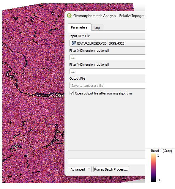
The Relative Topographic Position (RTP) is the free topographic index available in WhiteboxTools and is widely used in geomorphometric analysis to describe the relative elevation of each grid cell compared to its surrounding terrain. Instead of using absolute elevation values, this index evaluates whether a location is positioned higher or lower than its neighborhood, making it especially useful for identifying ridges, valleys, slopes, and flat areas.

The tool works by calculating the difference between the elevation of a target cell and the mean elevation of the surrounding cells within a user-defined moving window. Positive values indicate locations that are higher than their surroundings (such as ridges or hilltops), while negative values indicate lower positions (such as valleys or depressions). Values close to zero represent mid-slope or relatively flat terrain. This relative approach makes the index less sensitive to overall elevation and more effective for landform classification.

To compute the Relative Topographic Position in QGIS, open WhiteboxTools → Geomorphometric Analysis → Relative Topographic Position and select the input DEM. Two optional parameters control the scale of analysis: the filter X dimension and filter Y dimension, which define the size of the moving window used to compute local elevation differences. Smaller window sizes emphasize fine-scale landforms such as small ridges and channels, while larger window sizes highlight broader landscape features such as major valleys and uplands. Adjusting these parameters allows the user to analyze terrain structure at multiple spatial scales.

Figure 5: Relative Topographic Position Index (RTPI) Derived from the DEM

Landform Classification

Geomorphons

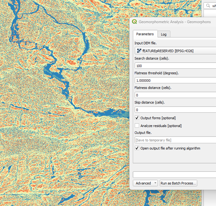
Geomorphons, also referred to as geomorphological phonotypes, are a method for classifying and visualizing landforms based on the relative elevation differences between a central grid cell and its surrounding neighborhood. Rather than relying on slope or curvature alone, this approach evaluates the local terrain pattern by analyzing elevation profiles in the eight principal directions (north, northeast, east, southeast, south, southwest, west, and northwest) around each cell. The algorithm compares the central cell to its surroundings to determine whether the surface is locally higher, lower, or similar in elevation, allowing the terrain to be categorized into typical landform elements such as ridges, valleys, slopes, flats, shoulders, and hollows. As a result, geomorphons provide an intuitive and spatially explicit representation of landform types and are particularly useful for automated landform classification and terrain segmentation. Geomorphons are particularly valuable in geomorphometric analysis because they transform continuous elevation data into meaningful, interpretable landform classes that can be used for landscape analysis, ecological modeling, hydrological studies, and terrain-based mapping

In WhiteboxTools, geomorphons can be computed by navigating to Whitebox Tools → Geomorphometric Analysis → Geomorphons. The primary input is a DEM. Several parameters control the scale and sensitivity of the analysis. The search distance defines how far the algorithm looks in each direction to detect elevation differences; increasing this value emphasizes broader landforms, while smaller values highlight fine-scale features. The flatness distance specifies the elevation tolerance used to identify flat surfaces—larger values result in more areas classified as flat. The skip distance allows the algorithm to ignore very near cells, reducing the influence of local noise or small artifacts. Together, these parameters allow the user to tailor the geomorphon output to the spatial scale and geomorphic characteristics of the study area.

The output raster encodes landform types using integer values, where each value corresponds to a specific geomorphic class defined by Whitebox (figure6)

Figure 6. Geomorphons-Based Landform Classification

In the resulting map, valley and pit classes clearly delineate drainage networks and depressions, while ridge and peak classes highlight topographic highs. Slopes, shoulders, and footslopes describe transitional zones between highs and lows, providing a comprehensive and intuitive landform classification.

Number of upslope or downslope neighboors

The Number of Upslope Neighbors and Number of Downslope Neighbors tools quantify local terrain shape by counting how many surrounding cells are higher or lower than a given grid cell in a Digital Elevation Model (DEM). These indices provide a simple yet effective way to describe surface form and local relief structure. The calculation is performed using a 3 × 3 moving window, where each cell is compared to its eight immediate neighbors. For the Upslope Neighbors tool, the algorithm counts how many neighboring cells have a higher elevation than the central cell. Conversely, the Downslope Neighbors tool counts how many neighboring cells have a lower elevation. The resulting values range from 0 to 8. A value of 0 indicates that all surrounding cells have the same elevation, corresponding to flat areas or uniform surfaces, while a value of 8 indicates that all neighboring cells are either higher (for downslope neighbors) or lower (for upslope neighbors), which typically represents peaks or pits depending on the context. These tools are useful for identifying peaks, pits, ridges, valleys, and transitional slope positions, and they provide a quantitative measure of local convexity and concavity. In WhiteboxTools, these parameters can be computed by navigating to Whitebox Tools → Geomorphometric Analysis → NumUpslopeNeighbors or NumDownslopeNeighbors. The only required input is the DEM, making these tools straightforward to apply and effective for exploratory geomorphometric analysis.

By combining these two parameters, the user can evaluate the degree of local convergence or divergence of the terrain. For example, in the left image, which represents the number of downslope neighbours, the red central band highlights an area where many surrounding cells are lower in elevation. This pattern typically corresponds to ridges or convex features, where elevation decreases in multiple directions away from the central cell. In contrast, the right image, representing the number of upslope neighbours, shows the same area with lower values, confirming that fewer surrounding cells are higher than the central cell. Conversely, areas with high upslope-neighbour values and low downslope-neighbour values indicate valleys or concave landforms, where surrounding terrain converges toward a lower central cell. Together, these complementary indices provide a simple but effective way to characterize local terrain shape and identify zones of topographic convergence and divergence.

Figure 7: Number of Downslope and Upslope Neighbours Derived from a Feature-Preserved DEM

Optional Process

Erosion Susceptibility Mapping

Geomorphometric parameters are most powerful when combined to support applied spatial analysis. As an optional extension of this tutorial, slope, curvature, and downslope index can be integrated to identify areas that are potentially more susceptible to surface erosion. This approach is particularly relevant for environmental studies, watershed management, and landscape stability assessment.

Erosion processes are strongly controlled by terrain steepness, surface curvature, and downslope connectivity. Steep slopes favor gravitational transport, concave surfaces concentrate flow, and areas with strong downslope connectivity enhance the acceleration of water and sediment. By combining these parameters, a relative erosion susceptibility map can be produced.

How to Do It in QGIS

The erosion susceptibility analysis begins by generating the slope raster (in degrees) using WhiteboxTools → Geomorphometric Analysis → Slope. Steeper slopes indicate a higher potential for erosive processes. Next, curvature is computed using WhiteboxTools → Geomorphometric Analysis → Mean Curvature, where negative values represent concave surfaces that tend to concentrate runoff. The downslope connectivity of the terrain is then quantified using WhiteboxTools → Geomorphometric Analysis → Downslope Index, which highlights areas where water and sediment can rapidly move downslope.

To combine these layers, each raster is first normalized using the QGIS Raster Calculator so that values range between 0 and 1. The operation are : slope_normalized=("slope@1" - SLOPE_MIN) / (SLOPE_MAX - SLOPE_MIN); Mean Curvature_normalized = (abs("curvature@1") - CURVABS_MIN) / (CURVABS_MAX - CURVABS_MIN); Downslope_normalized=("downslope@1" - DOWN_MIN) / (DOWN_MAX - DOWN_MIN); The normalized slope, curvature, and downslope index are then combined using a weighted linear model. A simple formulation assigns equal weights to each parameter, producing a relative erosion susceptibility index where higher values represent greater potential erosion risk. The resulting raster can be classified into low, moderate, and high susceptibility classes for interpretation and visualization.

Common Pitfalls and Best Practices

When conducting a geomorphometric analysis, several common issues can significantly affect the quality and interpretation of results. Digital Elevation Models may contain noise or artefacts, particularly in older or low-resolution datasets, and applying geomorphometric derivatives directly to such data can lead to misleading outputs; therefore, DEM smoothing should be performed prior to analysis. Care must also be taken with the Z conversion factor, as inconsistent vertical and horizontal units can distort slope, curvature, and related parameters. In addition, certain visualizations, such as grayscale aspect maps, may be difficult to interpret and should be symbolized using appropriate color schemes. Finally, individual geomorphometric parameters should not be interpreted in isolation; combining multiple metrics (e.g., slope, curvature, TPI, downslope index) provides a more robust and meaningful understanding of landscape structure and processes.

Beyond technical considerations, best practice in geomorphometric analysis also requires a strong emphasis on scale, context, and reproducibility. Many geomorphometric parameters are scale-dependent, meaning that window sizes, search distances, or filter dimensions must be selected in relation to the resolution of the DEM and the spatial extent of the study area; inappropriate scale choices can either oversimplify landforms or exaggerate local noise. It is therefore recommended to test multiple parameter settings and explicitly justify the selected values. Furthermore, geomorphometric outputs should always be interpreted in the context of regional geology, geomorphic history, and surface processes rather than as purely mathematical products. Documenting processing steps, parameter choices, and data sources is essential to ensure transparency and reproducibility, especially when results are intended for academic publication or decision-making. By combining careful preprocessing, thoughtful parameter selection, multi-metric interpretation, and clear documentation, geomorphometric analysis becomes a robust and scientifically defensible tool for understanding landscape structure and dynamics.

Conclusion

This tutorial demonstrated a complete and reproducible workflow for conducting a geomorphometric analysis using WhiteboxTools within QGIS, relying entirely on free and open-source software. Starting from a Digital Elevation Model, the methodology guided users through DEM preprocessing, noise reduction, and the extraction of key primary and secondary geomorphometric parameters such as slope, aspect, curvature, downslope index, geomorphons, and topographic indices. Each parameter was presented not only from a computational perspective, but also with an emphasis on geomorphic interpretation and visualization.

By integrating multiple geomorphometric derivatives rather than relying on a single parameter, the tutorial highlights how terrain structure, processes, and landform patterns can be quantitatively characterized in a robust and meaningful way. The use of feature-preserving smoothing, appropriate visualization techniques (hillshade, directional relief, hypsometric tinting), and careful parameter selection ensures that the derived outputs are both scientifically reliable and visually interpretable.

Overall, this workflow provides a transferable framework applicable to a wide range of disciplines, including geomatics, geology, environmental studies, geography, and hydrology. The tutorial equips users with practical skills to analyze and interpret topography, supports academic research and publication-quality outputs, and encourages best practices in geomorphometric analysis using modern, open-source geospatial tools.

Reference

Lindsay, J. B. (2016). Whitebox GAT: A case study in geomorphometric analysis. Computers & Geosciences, 95, 75–84. https://doi.org/10.1016/j.cageo.2016.07.003

Lindsay, J. B. (2023, March 25). Geomorphometric analysis tools. WhiteboxTools User Manual. https://www.whiteboxgeo.com/manual/wbt_book/available_tools/geomorphometric_analysis.html