Wind turbine location suitability

Introduction

With the growing expansion of the city Ottawa energy capacity requirements become an integral issue. Currently the Energy Ottawa Company supplies a majority of its energy to the city through what is known as the ‘run-of-the-river’ generating system. This is a series of small scale hydroelectric dam facilities spread out across the regions watershed (Energy Ottawa, 2010).

This method of energy generation is considered a green means of producing energy, as it does not typically involve emitting pollution into the atmosphere compared to coal, petroleum, or natural gas. What is often overlooked is the negative affects that hydroelectric dams pose to the health of watershed, impacting many aspects of both the natural and social environment. These adverse affects have caused the number of hydroelectric dams being built to be drastically reduced in Canada (Natural Resources Canada [NRC], 2009).

This has led many municipal and provincial governments to seek alternative green energy production techniques. As such wind energy has come to the forefront of this search. Wind energy is however not without its negative implications as well. Recent studies have been produced in which attribute the construction of wind farms as causing degradation the environment in sensitive areas, as well as possibly having negative implications to human health with prolonged exposure in close proximity to wind turbines. To mediate these concerns the provincial government of Ontario has released various restrictions, limiting areas in which the construction of wind farms is permitted.

Objective

The objective of this tutorial is to demonstrate a technique which identifies spatial regions deemed as potentially suitable locations for the development of wind energy production. This will display means for consideration of the restrictions imposed by the provincial government to evaluate the purposed region. The desire of this particular case is to identify suitable locations for wind energy production in Ward 21 of the Ottawa, Ontario region.

Restrictions

The Provincial Government of Ontario has provided the following restrictions in relation to the spatial placement of wind energy turbines for use of commercial applications:

• 135m from all existing public roadways

• 135m from all existing railway lines

• 1000m from all existing transmission lines

*These restrictions are relative to the turbine specifications of the Vestas V90, 3 megawatt model

These restrictions were provided by:

• Renewable Energy Approvals
• Technical Bulletin Six: Required Setbacks for Wind Turbines
• Drafted by the Environmental Registry March 1, 2010

Methods

The following will thoroughly demonstrate the techniques involved in this approach for identifying suitable wind energy production sites in the Ottawa city area. This example looks to specifically examine Ward 21, Rideau-Goulbourn.

Data Used

The first step is to gather all necessary data appropriate for the purpose of this exercise. This example uses vector shapefiles which include:

• Ottawa area boundary
• Ottawa city wards boundary
• Transmission lines
• Railways
• Federal Roads
• Provincial Roads
• Regional Roads

This data can be gathered at http://data.ottawa.ca/ or at http://geo1.scholarsportal.info

Software Used

The exercises demonstrated are completed using the Quantum GIS software interface. These are open source software materials which are freely accessible and available online. For new users it is suggested to use the standalone installer.

This is available by clicking this hyperlink. Click this!

This is based on the OSGeo4W packages and includes the newest version of qGIS (2.18.13) as well as the GRASS toolset.

Starting Map Project

1. Begin by opening the Quantum GIS software. Select ‘Layer’ from the drop down menu and open the ‘add vector layer’ function or click the ‘add vector layer’ icon on the toolbar. Ensure source type is set to ‘file’. Locate vector dataset by selecting ‘browse’ and open a shapfile which will be used for the project. Click ‘open’ and the shapefile will be added and displayed. Repeat this process until all shapefiles intended for use have added.
2. Once all vectors have been added, you should set the coordinate reference system (CRS). Select 'Layer' go to 'Set CRS of Layer(s)' and select which CRS you want.
   1. The recommended CRS is WGS 84, and when this is selected from the drop down menu, click OK and the layers you added are set with that CRS.
3. Next the vector files must be converted to GRASS vector layers.
   1. First open the GRASS toolbox by clicking the 'open GRASS Tools' icon.
   2. Click the 'module list' tab and open the 'v.in.org.qgis' tool.
   3. Under the 'options' tab select the layer to convert to GRASS under the 'ORG vector layer' heading.
   4. Name the output vector by typing a name into the 'name for output vector map' field (example: CityBoundary).
   5. Click 'Run' and wait for the output to successfully finish.
   6. Repeat this process for all vector files and close GRASS Tools.
   7. The original vector files may be removed from the map by right clicking them in the Layers Menu and selecting 'remove'.File:Vector to grass.bmp
4. The newly created GRASS vector layers should now be added. To do this select the 'add GRASS vector layer' icon on the toolbar.
   1. Select the location and mapset that were when the mapset was created.
   2. Under the Map Name field select the GRASS vector layers which to add.
   3. Repeat this process until all GRASS vector layers have been added.

Visualization of Restrictions using a Buffer

This portion will demonstrate how to imply a buffer region to each of the vector polyline layers representing limitations imposed by the spatial restrictions set by the Provincial Government of Ontario.

1. Open GRASS Tools
2. Select the module list tab and open the'v.buffer' tool.
3. To create the railway buffer, select the Railway Lines layer under the 'name of vector input map' field
   1. Set the 'Buffer distance along major axis in map units' field to 135 (this number represents the 135m restriction applied to Railways)
   2. Then set the name for output vector map (example: RailwayBuffer)
   3. Click Run, and wait for the output to successfully finish (this may take an extended period of time depending on the size of the input vector layer).
   4. Once the buffer has finished successfully click the 'view output' option to add the resulting layer to the map. File:Buffer tool.bmp
4. Complete this process for Road Layers again setting the 'Buffer distance along major axis in map units' to 135 as the restriction for roads is the same as railways.
5. When completing this process for the Transmission Lines layer make sure to change the 'Buffer distance along major axis in map units' parameter to 1000 to meet the 1000m restriction imposed to this infrastructure.

Representation of the Resulting Layers:

Creation of Total Suitable Areas Using Overlay

This section will demonstrate the use of vector overlay techniques in order to visualize total suitable areas free of spatial restrictions.

1. Open GRASS Tools
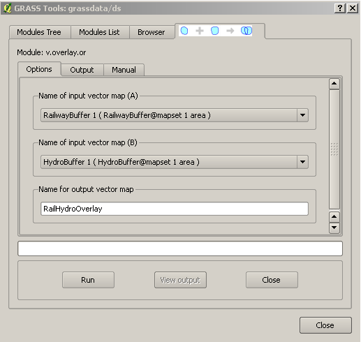
2. Under the module list tab open the 'v.overlay.or' tool.
   1. Under the 'input vector map (A)' field choose the Railway Buffer layer.
   2. Under the 'input vector map (B)' field choose the Transmission Lines Buffer layer.
   3. Under the 'output vector map' field provide an output name (example: RailHydroOverlay)
   4. Click run, and wait for the output to successfully finish. Click 'view output' to add the resulting layer to the map.
3. Return to the 'options' tab of the v.overlay.or tool.
   1. Under the 'input vector map (A)' field choose the overlay layer just created (example: RailHydroOverlay).
   2. Under the 'input vector map (B)' field choose the Roads Buffer layer.
   3. Under the 'output vector map' field provide an output name (example: TotalBufferOverlay)
   4. Click run, and wait for the output to successfully finish. Click 'view output' to add the resulting layer to the map.

This process results in the overlay of all three buffer restriction layers providing a total suitability layer which considers all restrictions.

Representation of the Resulting Layer:

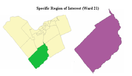
Narrowing Results to a Specific Delineation Area

This section focuses on narrowing the view to a specific area of interest. In this case the area of interest is Ward 21, Rideau. This is a largely rural/agricultural ward of the city making it a prospective optimal area for the production of wind energy. This process will involve the exporting of the specified area as a new shapefile as well as the use of an alternate type of vector overlay.

1. The following steps demonstrate the exportation of a specific area of interest as a new shapefile:
   1. Use the 'select features' tool select the area of interest.
   2. Next, right click the 'Ward Boundary' layer in the layer menu and select 'save selection as..'
   3. Set the format to 'ESRI Shapefile' and provide a new file name (example: ward21.shp). The projection will remain the same.
   4. Click 'ok'
   5. Add the newly created shapefile to the map project
2. Now a second form of vector overlay must be performed to add the suitable areas to the resulting area.
   1. To do this first open GRASS Tools
   2. Click the module list tab and open the 'v.overlay.and' tool
   3. Under the 'input vector map (A)' field choose the new specified area shapfile (example: Ward21).
   4. Under the 'input vector map (B)' field choose the suitable locations layer (example: TotalBufferOverlay).
   5. Under the 'output vector map' field provide an output name (example: Ward21SuitableAreas)
   6. Click run, and wait for the output to successfully finish. Click 'view output' to add the resulting layer to the map.

The output of this process will provide s suitable areas layer for the specific delineation region of interest.

Representation of the Resulting Layer:

Identifying Largest Suitable Area

The Largest suitable area can be identified using the 'measurement tool' located on the toolbar. Once the largest suitable area has been identified, create a new vector polygon to represent this area. This can be done using the 'create new GRASS vector tool'.

1. Select 'create new grass vector tool' on the toolbar
2. Enter an output name for the new vector layer (example: largest suitable area)
3. Create the new vector layer using the 'new boundary' tool

Representation of the Resulting Layer:

The resulting layer provides the largest suitable area for the specific region of interest with the consideration of all implied restrictions.

References

• Energy Ottawa. (2010). "Green Power". Accessed online: http://www.energyottawa.com/forms/index.cfm?dsp=template&act=view3&template_id=46&lang=e
• Natural Resources Canada. (2009). “Hydroelectric Generation”. The Atlas of Canada. Accessed online:http://atlas.nrcan.gc.ca/auth/english/maps/freshwater/consumption/hydroelectric/1