Supervised classification in QGIS
Contents
Purpose and Introduction
Every day thousands of satellite images are taken. To work with these images they need to be processed, e.g. they need to be classified. Since Remote Sensing software can be very expensive this tutorial will provide an open-source alternative: the Semi-automatic-classification plugin (SCP) in QGIS. The tutorial is going through a basic supervised land-cover classification with Sentinel-2 data. It is one suggestion to use the SCP. After running through the following workflow you will know the SCP better and you will be able to discover more opportunities to work with remote-sensing Data in QGIS. You can also find another tutorial about the SCP here [1]. Feel free to combine both tutorials.
Land cover classification allocate every pixel in a raster image to a defined class depending on the spectral signature curve. The classification will provide quantitative information about the land-use.
Installing the Software and SCP
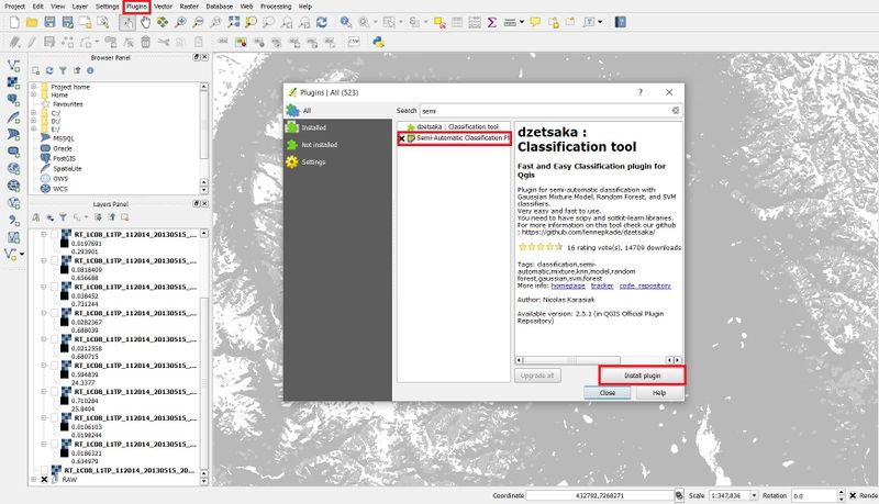
To start the tutorial you have to download the latest version of QGIS which is QGIS 3.4.1. "Bonn" and can be found here[2]. Make sure to download the proper version for your PC (34bit vs. 64bit). After installing the software the Semi-automatic classification Plugin (SCP) must be installed into QGIS. Navigate to the menu at the top to Plugin and select Manage and Install Plugins. Following the picture, the SCP can be found while typing "semi" in the search bar. Click install plugin and now you should be able to see the SCP Dock at the right or left side of your user surface.
Obtaining the Data
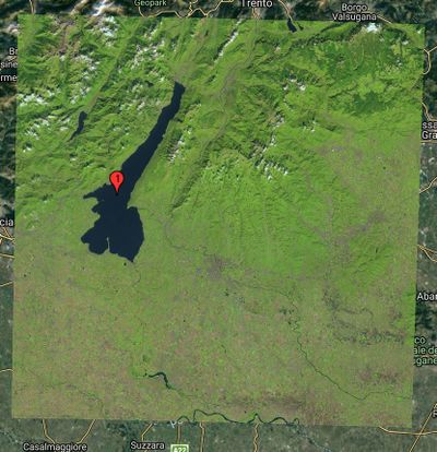
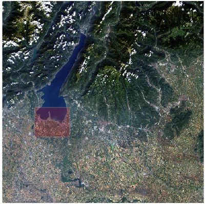
In this Tutorial, Sentinel-2 Data from the south of Lake Garda, Italy is used to run the classification. The data can be downloaded from the USGS Earth Explorer website here[3]. You can find an explanation how to download data from the Earth Explorer in the tutorial Remote Sensing Analysis in QGIS. To find the same picture as used in this tutorial, search for Lake Garda and select the time period from August to October 2018. Among Data Sets select Sentinel-2 and you should find the following picture:
ID: L1C_T32TPR_A008056_20180921T101647 Date: 21st of September 2018.
It is always easier to work with cloud free pictures, otherwise you have to use a cloud mask.
Unpack the Data
The downloaded data is packed in a zip-File. Therefore, you have to unzip the Data before working with it. Afterwards you can find the image data in your home directory under GRANULE → L1C_T32TPR_A008056_20180921T101647 → IMG_DATA. For each band of the satellite Data there is a separate JPEG file.
Load the Data into QGIS and Preprocess it
To load the data into QGIS navigate to Layer at the top your user surface. Choose Add Layer, and then Add Raster Layer.... You should see the Data Source Manager now. Leave "File" selected like it is in default. Under Datasets you can navigate to the directory described above where you find the imageries. Make sure to load all JPEG files into QGIS except the file of band 10: T32TPR_20180921T101019_B10. Band 10 is the Cirrus band and is not needed for this approach.
Creating a Band set
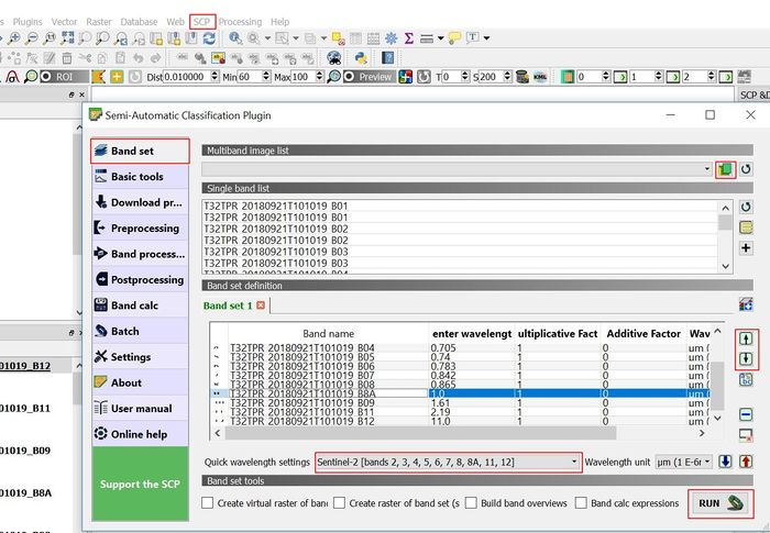
The next step is to create a band set. Navigate to the SCP button at the top of the user surface and select Band set. Under Multiband image list you can load the images into SCP and then into the Band Set 1. Select Sentinel-2 under Quick wavelength units. As you see, the layers have numbers (e.g. B01) which are the band numbers. Make sure the bands are in the right order and ascending. The picture below should help to understand these steps.
If you do not want to see a gray scaled image navigate to the SCP toolbar at the top of your surface to RGB and choose 4-3-2 to see true colours.
Clip the Data
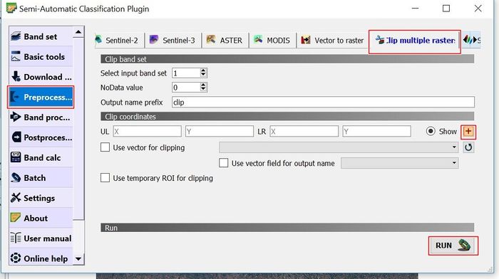
Since the area of the picture is very large it is reasonable to work with just a section of the image. Therefore, the SCP allows us to clip the data and only work with a part of the picture. Navigate to the SCP button at the top of the user surface, under Preprocessing you find clip multiple Raster. Your surface should look similar like in the picture below. Choose Band set 1 which you defined in the previous step.
To clip the data press the orange button with the plus. Minimize the SCP window and you can now define the area you want to work with while clicking with the right button on your mouse. I suggest to define an area south of the mountains to avoid dealing with mountain shadows in the classification. In addition, in the south of the picture the scenery is cloud-free. For instance, choose an area like this:
After defining the section under Clip coordinates there should occur numbers. Click run and define an output folder. In the Layer Dock, for each Band (1-9,11,12) a separate resized Raster Layer occurs.
Automatic Conversion to Surface Reflection
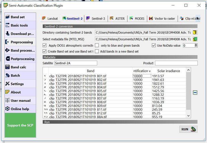
The last preprocessing step is to run an atmospheric correction. Go to SCP, Preprocessing, Sentinel-2 and choose the directory where you saved the clipped data. Check Apply DOS1 atmospheric correction and uncheck only to blue and green bands likely in the sample picture. Since a new band set is needed, it is useful to check Create band set. The solar radiance should be recognized automatically. Click run and define an output folder.
The output files will be named e.g. like this: RT_clip_T32TPR_20180921T101019_B03.
Supervised Classification
We can now begin with the supervised classification. Make sure you see the SCP & Dock at your surface. If not, clicking this button in the tool bar will open it.
Set Region of Interests (ROI)
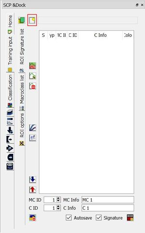
First, you must create a file where the ROIs can be saved. To do so, click this button:
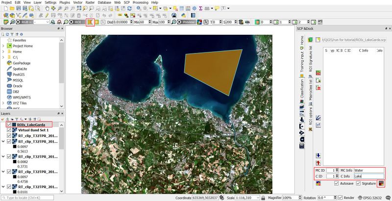
Click the Create a ROI button to create the first ROI. You can define the ROI with mouse clicks, to complete it, click right.
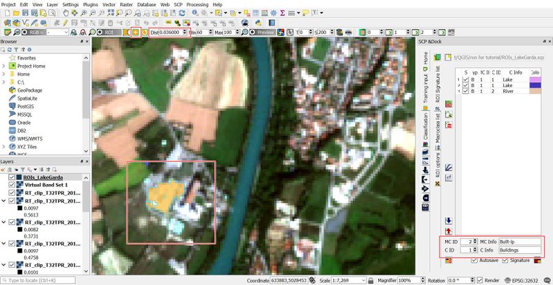
In the following picture the first ROI is in the lake. You can see that the macro class (MC ID) is named Water and the subclass (C ID) Lake. In this tutorial, only the macro classes will be significant, since it is a basic classification with only four different classes. If you want to have more specific classes you can use the subclasses. Save the ROI.
A second option to create a ROI is to activate a ROI pointer. This can be done while clicking the plus in the red box (see the following picture) and defining the radius where the SCP should look for similar pixels. This tool makes it faster to set ROIs. Your ROI could look like this:
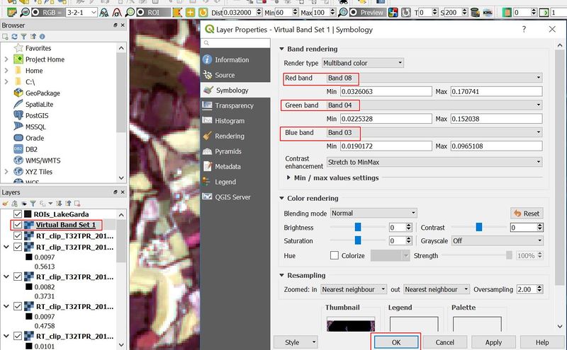
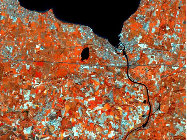
In this tutorial 4 macro classes will be defined: water, built-up area, healthy vegetation, unhealthy vegetation. Since vegetation is reflecting light in NIR (Near infrared), we can visualize it in an image with false colours and therefore distinguish between healthy and unhealthy vegetation. To do so, click right on the layer Virtual Band Set 1 and choose Properties. Define Band 08 (NIR) as red, Band 04 (Red) as green and Band 3 (green) as blue like in the image below.
Now, the healthy vegetation occurs red while the unhealthy vegetation (e.g. unused fields) occurs blue/grey.
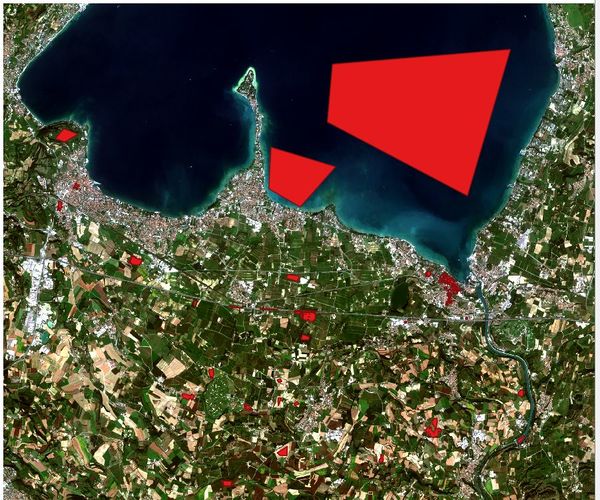
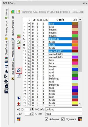
Keep going setting ROIs for unhealthy and healthy vegetation. Try to be as accurate as possible, to make sure that pixels are assigned to the proper class. In the following picture an example of several ROIs is shown:
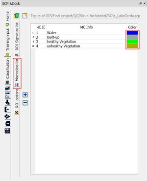
Before we run the classification we can change the colours of the macro classes in the SCP Dock. Click Macroclass List and double-click on the colour fields:
Choose an appropriate colour for every class.
Running the classification
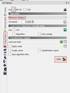
Now go to the Classification window in the SCP Dock. You will notice that there are various options to run the classification. For instance, there are different classification algorithms: Minimum Distance, Maximum Likelihood or Spectral Angle Mapper. Feel free to try all three of them. It always depends on the approach and the data which algorithm works the best. If you check LCS, the Landcover Signature classification algorithm will be used. If you uncheck it, the chosen algorithm above will be used. In the classification of this tutorial, the Minimum Distance Algorithm and Spectral Angle Mapping came out as the best classification algorithms.
Check MC ID to use the macro classes and uncheck LCS. Click run and safe the classification in your desired directory. If areas occur unclassified go back and set more ROIs.
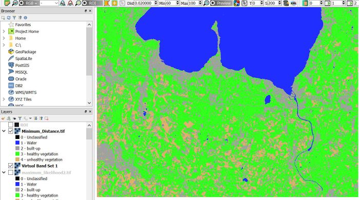
The output can look like this:
Assessing the classification
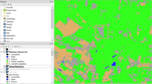
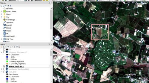
You can assess the classification easily with your eyes. You can move the classification Layer above the Virtual band Set 1. Zoom into the picture and focus on an object. Checking and unchecking the classification layer allows you to verify the classes. As you see, it is difficult for the program to distinguish between unused fields and buildings.
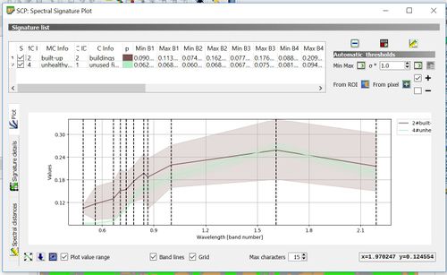
The following picture explains why the two classes are mixed up sometimes.
Built-up area (brownish line) and unhealthy vegetation (turquoise line) have very similar spectral signature plot and the algorithm refers to these signatures. However, you can reduce this error by setting more ROIs. Another possibility would be to include Indices in the classification which are explained in the Tutorial mentioned above (Remote Sensing Analysis in QGIS). Unfortunately, you can not totally overcome the error.
You can visualize the spectral signature for every ROI. For this select the ROIs you want to visualize and click Add highlighted signatures to the signature plot.
The SCP provides a lot of options to achieve a good classification result. It depends on the approach, how much time one want to spend in improve the classification. The SCP provides even more options to improve the ROIs while altering the spectral signatures for different classes. Nonetheless it will not be possible to classify every single pixel right.
Calculate the Kappa Coefficient
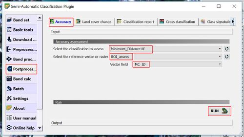
A quantitative method to assess the classification is to calculate the Kappa Coefficient. First, you have to create a new layer with ROIs and set again ROIs for the four classes to have a reference ground. You can not use the ROIs you used for the classification because you want to compare the classification with undependable training input. After you created various ROIs open the SCP and go to Postprocessing, Accuracy. As your input layer choose your best classification result. The reference raster layer will be the new ROIs you just set:
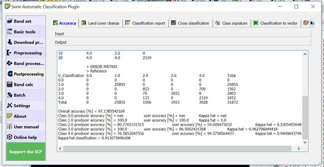
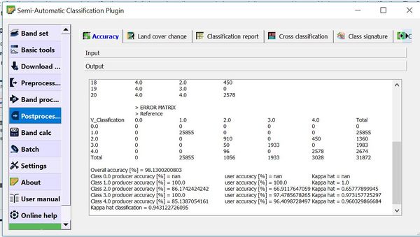
The output will tell you the accuracy for each class and the overall accuracy. The Kappa scale is from 0 to 1, 0 means the classification is not better than random, 1 means the classification is highly accurate.
In the first picture you see the assessment report of the Minimum Distance algorithm and on the second the one from the Spectral Angle Mapping. Comparing both the overall Kappa Coefficient of the Spectral Angle Mapping is a bit higher (0.943) than the one of the Maximum Distance (~0.913). However, both overall Kappa Coefficients values are very high. This is questionable and probably because too little ROIs were set in the second ROI ground reference Layer.
Conclusion
The tutorial showed one possible remote sensing workflow in QGIS and also provides a introduction into the SCP Plugin and hopefully motivated you to try out more. You can find more Information about the Plugin here [4] and discover more tools the SCP offers.
