Flood Risk Assessment in QGIS

Introduction

Flood assessment is one of many important purposes for which GIS capabilities can be applied in a practical manner. The scope of the analysis in the tutorial includes a portion of the downtown core of the Ottawa-Gatineau area. This analysis is particularly relevant due to the high number of flooding events and high-rainfall in Ottawa. By completing flood risk assessments, the city can identify at-risk buildings/populations, as well as develop stronger preparedness measures for when a flood does occur.

The purpose of this tutorial is to provide users with an introduction/guidance in completing a flood risk assessment, as well as an introductory glance into QGIS.

Software Requirements

In order to begin this tutorial, you will need to download the QGIS software package from the following link (https://www.qgis.org/en/site/ ). This tutorial was created using QGIS version 3.8.1 and is available for Windows, MacOS X, Linux and Android.

All steps of the tutorial will be completed using this free and open source software, and will not rely on the use of any other programs.

Data

The primary source of data used for this analysis will be the High Resolution Digital Elevation Model (HRDEM) - CanElevation Series, produced by Natural Resources Canada for the city of Peterborough. The dataset is hosted on the Open Data Canada website here: (https://open.canada.ca/data/en/dataset/957782bf-847c-4644-a757-e383c0057995).

There are two main types of elevation datasets provided as part of the High Resolution Digital Elevation Model (HRDEM). Both datasets have been derived from airborne LIDAR data. The two datasets are in the form of a Digital Surface Model (DSM) dataset and a Digital Terrain Model (DTM) dataset. It is important to know the difference between these two elevation datasets and how this can affect your analysis of flooded areas.

A Digital Surface Model or DSM is very similar to that of a Digital Elevation Model (DEM) or Digital Terrain Model (DTM). All three show elevation data about the earth’s surface. One major distinction between a DSM and a DTM is the presence of man-made and natural features. This means the DSM shows the tops of buildings, houses, highways, tree canopies, vegetated surfaces and all manor of other solid features above the surface of the ground. They are traditionally in the form of a raster image. DSM’s are generally used for purposes where it is necessary to see objects protruding from the surface of the earth. This includes tasks such as assessing the encroachment of vegetation or viewshed analysis for a new Highrise. They are not used for hydrologic modelling such as flood analysis.

A Digital Elevation Model or DEM does not include features that protrude from the ground. A DEM represents the ground elevation from sea level. It therefore does not include the tops of trees or buildings. This is very useful for the purpose of hydrologic mapping, such as flood analysis. DEM’s are generally in the form of a raster image.

A Digital Terrain Model or DTM can have varying definitions. In some cases, Digital Terrain Model and Digital Elevation Model are used interchangeably. This means that the dataset would be a raster image of the Earth’s surface excluding buildings and vegetation. In other cases, a Digital Terrain Model can be essentially a DEM represented through point data. The dataset shows the elevation of the earth’s surface through a series of equally spaced points. These points have an associated x and y value along with a third value for elevation. In this case the DTM would be in the form of a vector dataset, such as a shapefile.

The DTM dataset available through the High Resolution Digital Elevation Model link is in the form of a geotiff (.tif). This means it is essentially the same as a DEM and can be used for flood mapping analysis. The DTM data that we will be using in this analysis will be at a resolution of 1m and will be projected in the UTM NAD83 (CSRS) coordinate system.

Additional vector data will also be used in this analysis from the Peterborough Open Data Hub. This includes building footprints, roads, pedestrian footpaths and hydrography polygons.

• See next section for instructions on how to download the files.

Downloads

Peterborough Digital Terrain Model Data

High Resolution Digital Elevation Model (HRDEM) - CanElevation Series

The High Resolution Digital Elevation Model (HRDEM) - CanElevation Series dataset hosted on the Open Canada Data web portal, where you can download different sets of DTM and DSM data across Canada

1. Click on the following link

2. Use the find function (Ctrl + F) to find each of the three images listed below.

1m_utm17_e_20_90

1m_utm17_e_21_90

1m_utm17_e_21_91

3. Download each file into a folder on your computer.

Peterborough Vector Data

This data is hosted by Peterborough's GIS Open Data initiative on their Open Data web portal.

1. Click on the following links and download the data as .shp files (a .zip file will be downloaded)

Hydrography Polygons: link This is a polygon of all the waterways in Peterborough.

Buildings: link This is a polygon layer of all the building footprints in Peterborough.

Roads: link This is a line layer of all the road networks in Peterborough.

Pedestrian Network Polygon: link This is a polygon layer of all the pedestrian footpaths and bike trails in Peterborough.

2. Go to the .zip files you previously downloaded and extract them to the same folder as you Peterborough DTM data.

QGIS Methods and Instructions

Importing and Merging

Step 1.

• Upload the .tif files into QGIS by navigating through the Browser window.
• Select the folder where your files are saved, (can be added to favourites by right clicking the folder) and drag in all four .tif files to the main window.
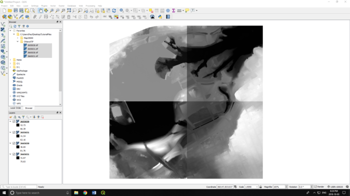
• The result should be the four raster images together in a square, as pictured below:
  • Note: If images are too hard to read, clicking on the image twice will result in a larger version of the image.

Step 2.

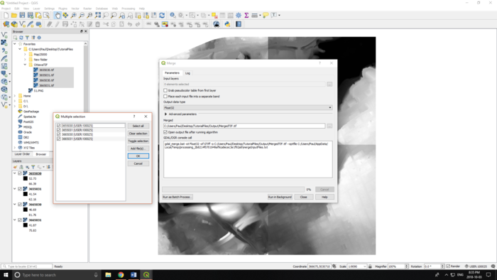
• Use the merge tool (Raster -> Miscellaneous -> Merge) to combine the .tif files into one working layer feature.
• In the merge tool, select the four .tif files through the Input Layers selection, directly under the Parameters tab.
• Once the layers have been selected, click Run in Background in order to merge the files.
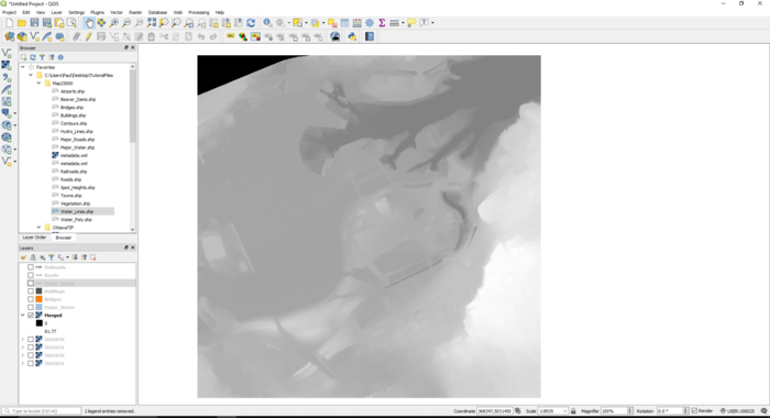
• The resulting merged file should look similar to the image below:

Using the Merge tool.

Merged raster files.

Creating an AOI

Step 3.

• At this stage an Area of Interest will be created, so we can clip our Ottawa layers in the next step.
• Navigate to Layers -> Create Layer -> New Shapefile Layer
• At the top of the window, give a name to your new file (AOI is suitable), and select Polygon as the Geometry Type -> At this point a new layer named AOI will be created.
• Right click on the newly created AOI layer, and select Toggle Editing. Once this is selected, navigate to the top panel and find the Add Polygon Feature icon (it looks like the green of a golf course).
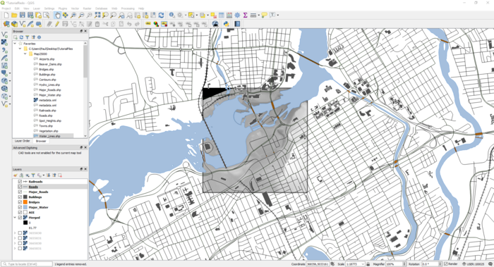
• Do your best to draw a border around the Merged layer (hint: use your numpad to move your screen when zoomed in), when complete, right click on the screen and when prompted to save changes to the layer, select Yes.
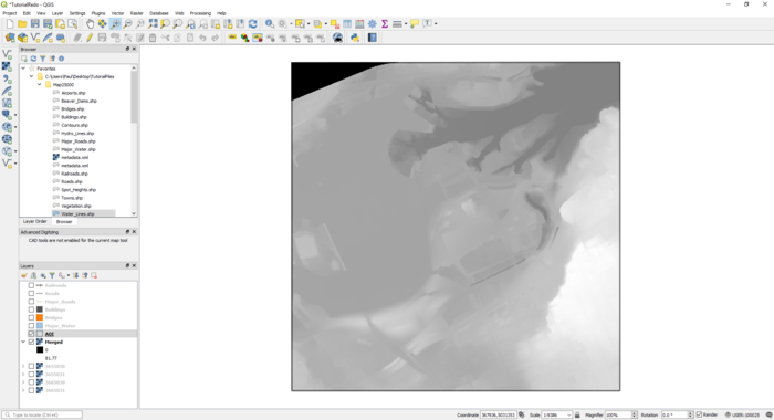
• The final step of creating an AOI is to right click on the icon/symbology for the layer, and select border. The final AOI and Merged layer should look similar to what is shown below:

Vector Layers & Clipping

Step 4.

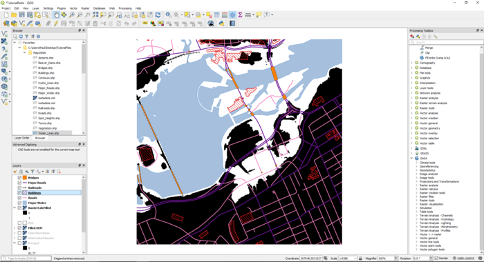
• Once the four raster images have merged, and the AOI has been created around it, the City of Ottawa files that were downloaded earlier can be added into QGIS.
• Navigate to the folder they were saved in (same process as importing the .tif files) and drag in the features (vector data) that you want displayed.
• For the purposes of the tutorial, the polygons used were: Major Water, Buildings, Roads, Major Roads, Railroads, and finally Bridges.
• Ensure the polygons are overlaying the merged raster layer, and edit the appearance of each feature as you want (double click on the icon to the left of each layer name).
• The resulting file should appear similar to the image presented below:

Step 5.

• Now that everything we want is added, the vector layers can be clipped to match the extent of the merged raster layer.
• Navigate to Vector -> Geoprocessing Tools -> Clip
• Select the layer you want to be clipped as the Input Layer, and the AOI as the Clip Layer. This clips all parts of the vector layer that is outside the area of the clip layer (the AOI).
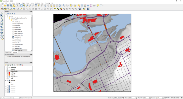
• Repeat this process until all the City of Ottawa vector layers have been clipped, renaming each newly created layer as "name" clip, or by removing the original layer and reassigning the name to the clipped layer.
• When all the vector layers have been clipped, the result should look similar to this (remember to symbolize everything that has been clipped):

Sink Fill

Step 6.

• In this step, the Sink Fill (Wang & Liu) was used from the QGIS toolbox. This was used in order to fill any spatial outliers that may have an effect on the overall result of the flood risk assessment.
• Navigate to Processing at the top of the program, and from there select Toolbox, in order to open the list of available tools.
• At the bottom of the list of tools is SAGA, select this and continue down until you reach Terrain Analysis - Hydrology -> Fill Sinks (Wang & Liu)
• Under the dropdown list for DEM select the layer Merged, and select Run (it's also a good idea to save Filled DEM to an Output folder in your primary directory).
• Upon completion, move your mouse to the layers area, and move the three new layers (Filled DEM, Flow Directions and Watershed) underneath the vector layers.
• The final output will look the same as the image in Step 5, if everything has gone correctly.

Raster Calculator

Step 5.

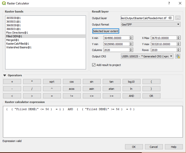
• Raster Calculator is used in this step to establish what areas will be flooded given an increase in water level of 1 meter -- visualized in the example is an increased water level of 1m.
• Navigate to: Raster - Raster Calculator.
• Use the Raster Bands and Operators to recreate the following expression: ( ( "Filled DEM@1" <= 56 ) = 1 ) AND ( ( "Filled DEM@!" >= 56 ) = 0 )
• If entered correctly, Expression Valid will appear under the expression window, and a new new layer will be created.

Results

Step 6.

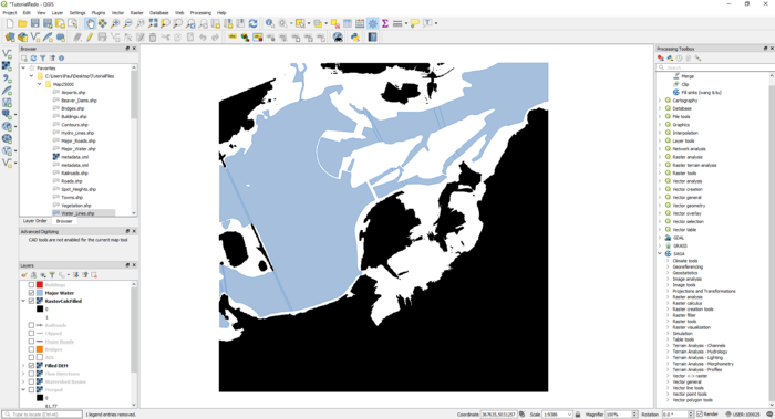
• Upon completion of the raster calculator, an output of the Ottawa-Gatineau downtown area will be given (same extent we have been working with the entire time).
• The areas that will be flooded given a rise in water levels of ~ 1 meter are in white (1), while the areas that are untouched remain black (0).
  • Note: The image below has all other layers hidden in order to see the specific area that will be flooded. In order to determine what infrastructure will be affected (and make use of the previous steps), it is important to add all layers back, as seen in the next step.

Step 7

• At this stage the flood analysis is almost complete, but we want to visualize and demonstrate what has been affected by the rising water levels. Simply turn all infrastructure layers back on (i.e. Buildings, Roads).
• If not visible, move the layers to the top of the Layers tab/window by dragging them above the layer RasterCalcFilled (if not renamed).
• Finally, make adjustments to the symbology (right-click the layer name, Properties, Symbology) and use something that demonstrates if the infrastructure is flooded or not, such as an outline.
• The final output should look similar to the image below:

References

Schuurman, N., Bell, N. J., L'Heureux, R., & Hameed, S. M. (2009), "Modelling optimal location for pre-hospital helicopter emergency medical services" BMC Emergency Medicine, 9, 6. [1]