Generating Wetness Indices for Watersheds in GRASS

GENERATING WETNESS INDICES FOR WATERSHEDS IN GRASS

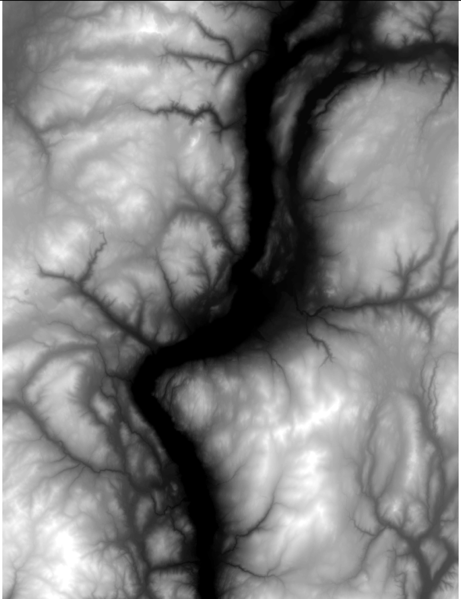
This tutorial will illustrate the processes involved in generating a topological wetness index from a digital elevation model using GRASS modules through Quantum GIS. Each step involved in generating a wetness index for a watershed will de explained, and example maps from a sample analysis will be provided. In the sample analysis, a wetness index was generated for the Carp River watershed in Ottawa, Ontario using a DEM of the Ottawa-Gatineau region (Fig.1).

Once the DEM is loaded in QGIS, create a GRASS mapset with an appropriate projection and workplace extent. Using r.in.gdal.qgis, import the DEM into the new mapset.

1.0 BACKGROUND INFORMATION: In hydrology, a watershed refers to an area of land in which all the precipitation runoff drains into a common waterway, such as a lake, river, or ocean. Therefore, drainage basins act as natural funnels, collecting the precipitation that lands within their borders, and directing it into the common waterway outlet. Watersheds are arranged in hierarchical order, where the size of a given watershed is determined by the location of its outlet. Therefore, as the outlet of the watershed moves downstream the watershed becomes larger, and consists of more sub-watersheds. In hydrology, watersheds are extremely important since they delineate regions that contribute to flow in a given waterway.

Wetness indices are used to describe spatial moisture patterns within a given region. They are calculated based on a region’s contributing upslope area and slope, where areas with low slope and large contributing area are expected to be relatively wet and areas with high slope and small contributing area are expected to be relatively dry. When a wetness index is calculated for a given region, the index should be calculated for the entire watershed in which that region is located, in order to ensure flow accumulation accuracy. In the sample analysis, wetness index was calculated for the Carp watershed based on [WetnessIndex=ln(A/tan(B))] where A represents the upslope contributing area and B represents slope.

2.0 GENERATING WATERSHED BOUNDARIES: In order to identify the spatial extent of the watershed of interest, use r.watershed to generate an image of watershed boundaries across the DEM. The r.watershed module uses the DEM and a threshold parameter as input. In this case, the threshold parameter refers to the minimum size in cells a watershed must be for it to be delineated. It may take some experimentation to acquire a proper threshold parameter that will produce watershed boundaries that correspond with the watershed outlet that was chosen in your research. Once the watershed boundaries are output, use them to focus the GRASS extent around the watershed of study (Fig.2). This will reduce processing times and eliminate extraneous data from calculations and visual representation.

In the sample analysis, watershed boundaries were delineated based on [r.watershed elevation=DEM threshold=10000 basin=Watersheds]

2.1 GENERATING A WATERSHED MASK: In order to make images watershed-specific, a mask for the watershed of interest is required. In this case, the mask is used to prepare images for visual display, and to eliminate extraneous data in output images, allowing for proper color schemes to be used. In r.mapcalc, generate a mask for the watershed of interest based on [r.mapcalc WatershedMask=if (Watersheds==24] Where 24 is the cell value representing the Carp watershed in the watersheds map.

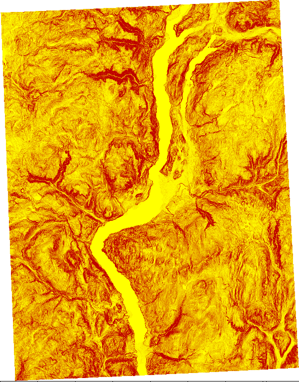
3.0 GENERATING SLOPE MAPS: To generate slope maps of the watershed that will be used to calculate wetness index, use the r.slope.aspect module. Report the input DEM and output slope-map names, and set the format by which the module reports slope (important depending on the wetness index equation that will be used). In the sample analysis, slope maps were set to report slope in degrees. Slope maps were generated based on [r.slope.aspect elevation=DEM slope=Slope format=degrees].

3.1 ELIMINATING ZERO SLOPE AREAS: Since slope appears in the denominator of the wetness index equation, regions with slope values of 0 will result in undetermined results for wetness index. To avoid null areas in the wetness index images, cell values of 0 should be assigned a value of 0.0001. To eliminate cells with a value of 0, use r.mapcalc to multiply the mask of the watershed by 0.0001. The slope mask is generated based on [r.mapcalc SlopeMask = WatershedMask*0.0001]

Next, in r.mapcalc, add the slope image and the slope mask together. This will replace values of 0 degrees with values of 0.0001 degrees, while producing only a negligible increase in slope in all other areas. In the sample analysis, the final slope map was generated based on: [r.mapcalc Slope_wNoZeros = Slope + SlopeMask]

The slope image, and the color scheme used to display the image, is illustrated below in Figure 3, and Table 1, respectively. Note that in Figure 3 the slope image has been multiplied by the watershed mask for visual display.

4.0 GENERATING ACCUMULATED FLOW MAPS: To generate maps of accumulated flow, use the r.watershed module. The same threshold parameter that was originally used to delineate the watersheds should be used to generate accumulated flow. In the sample analysis, accumulated flow maps were generated based on [r.watershed elevation=DEM threshold=10000 accumulation=AccumFlow].

The accumulated flow image, and the color scheme used to display the image, is illustrated below in Figure 4, and Table 3, respectively. Similar to Figure 3, the accumulated flow image has also been multiplied by the watershed mask for visual display.

5.0 GENERATING WETNESS INDEX MAPS: Using the slope and flow accumulation maps from Sections 2 and 3, calculate the wetness index of the watershed using r.mapcalc. As discussed earlier, wetness index is calculated based on a region’s contributing upslope area and slope, where contributing upslope area is calculated by multiplying the flow accumulation image by the cell size. In the sample analysis, wetness index was calculated based on [r.mapcalc WetnessIndex = log(((AccumFlow*AREAcell)/tan(Slope)), 2.718281828)]

The wetness index image, and the color scheme used to display the image, is illustrated in Figure 5, and Table 2, respectively. Finally, the image was multiplied by the watershed mask.

5.1 STANDARDIZING WETNESS INDEX MAPS: A common approach when comparing wetness indices is to standardize values between 0-1. If the wetness index image is going to be compared with other indices, standardize index values using r.mapcalc and r.info. Standardized wetness images can be generated based on [r.mapcalc WetnessIndex_Standardized= ((WetnessIndex – minWetnessIndex)/(maxWetnessIndex – minWetnessIndex))].

6.0 USER DEFINED COLOR RULES: Due to large flow values in rivers, streams, and creeks within the watershed, flow accumulation and wetness index maps are often ‘washed out’ due to poor color schemes. To allow proper interpretation of these maps, generate user defined color rules based on the distributions of values in the map. To acquire distributions, use r.stats –c to view the counts of each value that exist in the image, or use the histogram function provided for gdal rasters in QGIS. Apply color rules in r.colors based on [r.colors map=FlowAccum rules=c:/CarpWatershed/Location/Mapset/FlowColors.txt]

7.0 FILTERING THE DEM: In order to achieve a specific level of detail in the final wetness index image, filtering the DEM prior to generating the slope and flow accumulation maps may be required. Filtering can also reduce errors in future output maps that are caused by the DEM, or how the DEM was created. By limiting filtering to the DEM only, all output maps are derivatives of a specific elevation model. For example, a slope output image from a filtered DEM represents slopes in that specific DEM. However, if the slope image was filtered after output, it would be difficult to tell what DEM the slope image is reporting slope for. 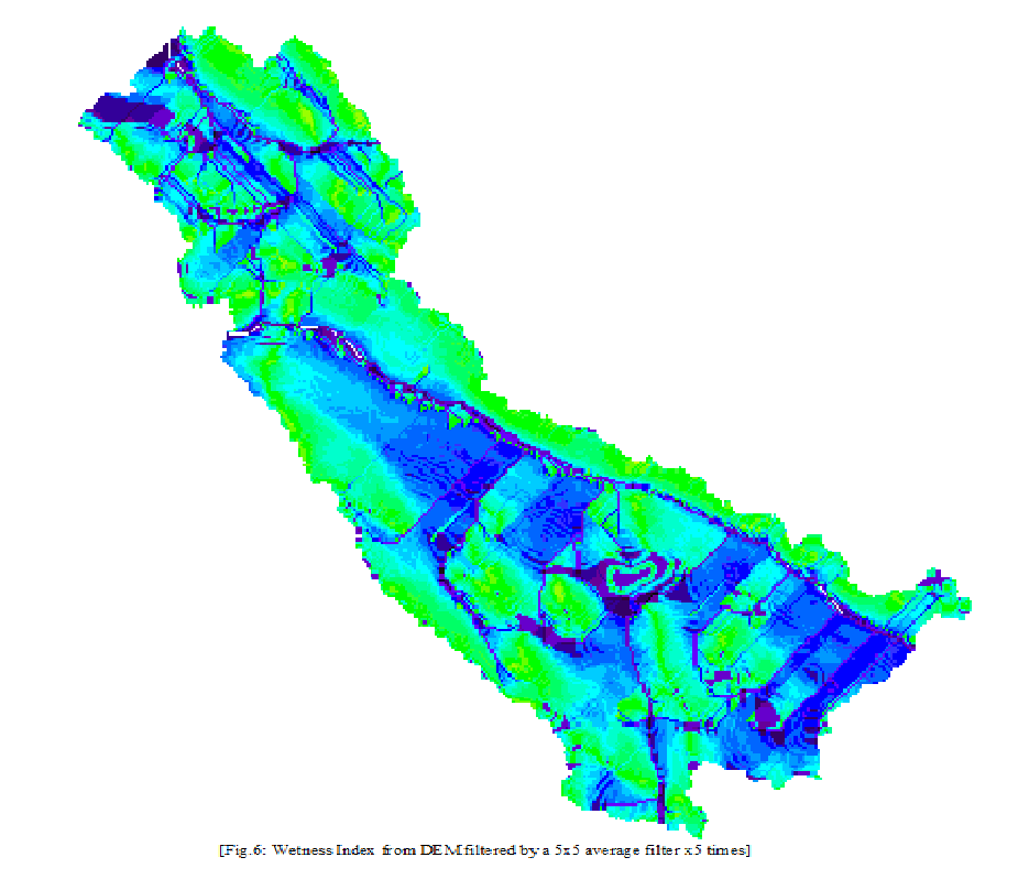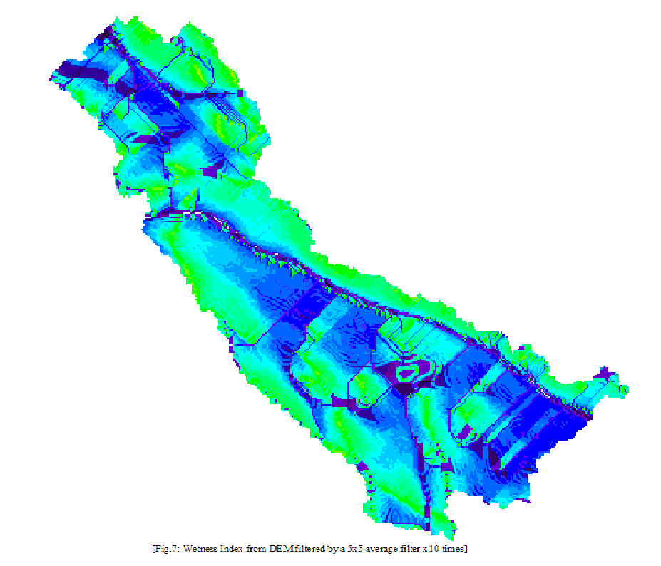The type of filter that is applied to the DEM, and the number of times the filter(s) are run, will have large effects on both the appearance and usability of slope, flow accumulation, and wetness index images. Generally trial and error is required to find the proper series of filters to produce the desired level of detail, and ‘smooth’ the DEM enough to reduce future errors in output maps. In the sample analysis, filters were applied to the DEM based on [r.mfilter input=DEM output=DEM_filtered filter= ‘path to filter file’ repeat= ‘number of repeats’].

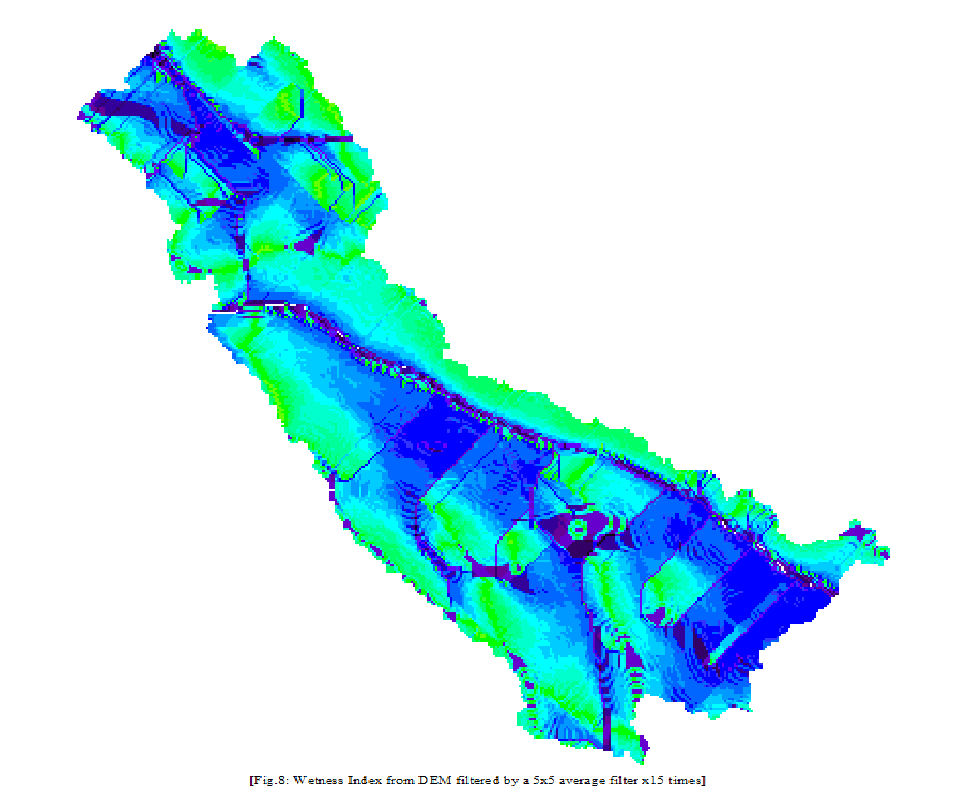
Figures 6, 7, and 8 show wetness index images that were generated from a DEM that was filtered a varying number of times with a 5x5 average filter. All images have the same scale as the wetness index image in Figure 4.

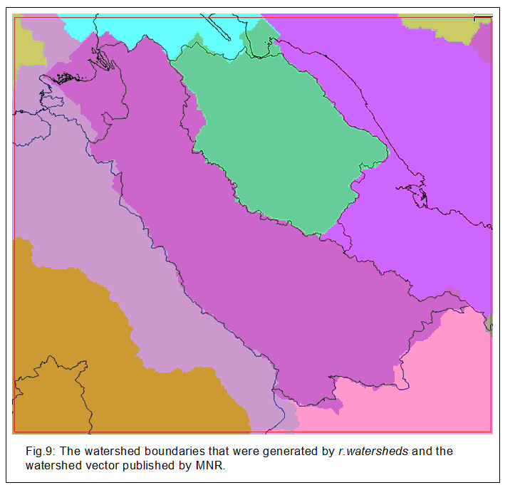
8.0 VERIFYING OUTPUTS: 8.1 VERIFYING WATERSHED BOUNDARIES: To assess the accuracy of the watershed boundaries output, obtain digital maps (either raster or vector) of verified watershed boundaries from local conservation authorities. This will allow visual and statistical comparison of the output watershed and the verified watershed boundaries. In the sample analysis, watershed boundaries were compared to a watershed boundary vector file that was published by Ministry of Natural Resources. The two sets of watershed boundaries are illustrated in Figure 9.

Based on the watershed comparison, r.watershed delineated the Carp watershed fairly accurately in the southern and mid portions of the region. However, in the northern portion of the watershed delineation was inaccurate due to a variety of potential errors. One potential source of error is the use of an inappropriate threshold parameter in r.watersheds while delineating watersheds. Another potential source of error is the possibility that Ministry of Natural Resources used a different DEM, different DEM preprocessing methods, or different software when generating the watershed boundaries.

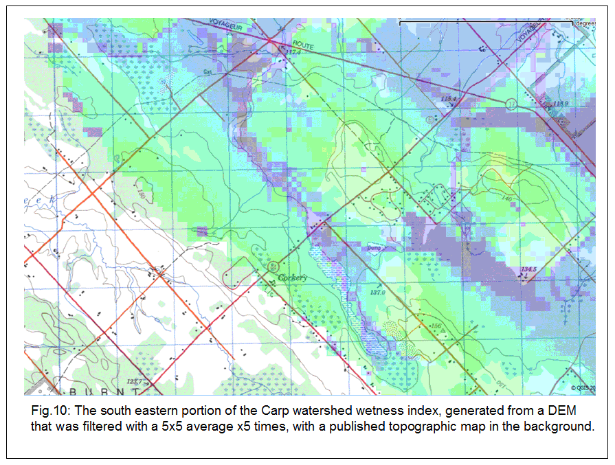
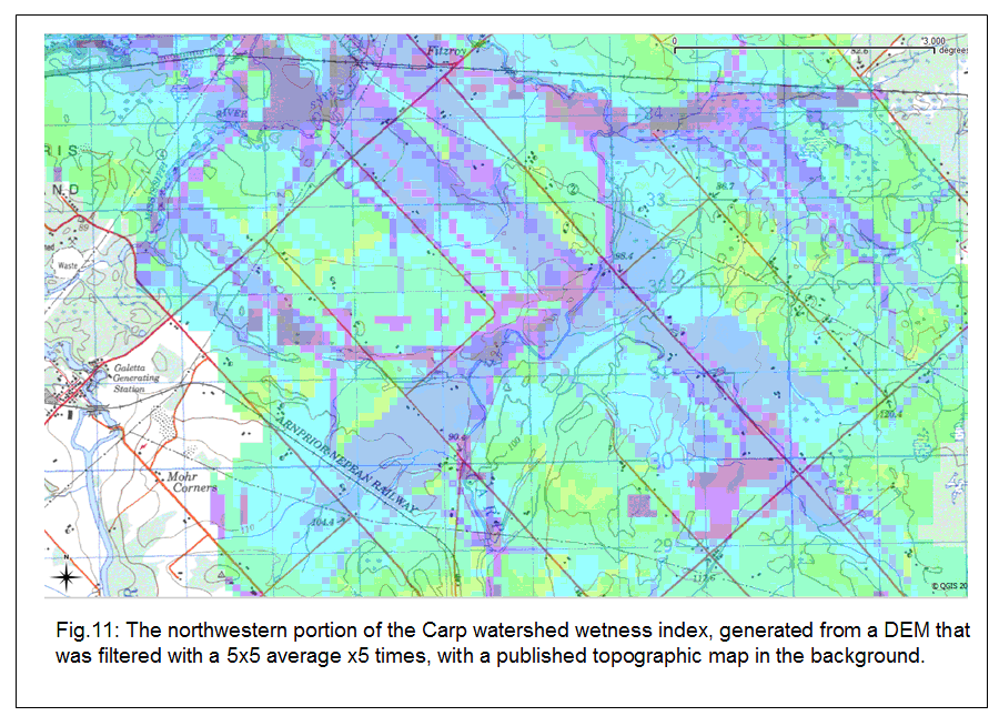
8.2 VERIFYING WETNESS INDEX: If digital topographic maps are available, they provide a good means to evaluate the potential accuracy of output wetness index images. With wetness index and topographic maps on screen, explore relatively wet areas on the wetness index image. Based on the landscapes that are reported by the topographic map, evaluate the accuracy of the wetness index image. In the sample analysis, the wetness index display in QGIS was set to be ~50% transparency. A topographic map covering the extent of the watershed was placed behind the wetness index image. Figures 10 and 11 illustrate screenshots during verification. The wetness index image in Figures 10 and 11 use the same color scheme as those in Figures 5, 6, 7, and 8, however since the image is set to be partially transparent, colors appear washed out.

Based on Figures 9 and 10, the wetness index map seems to be accurate in identifying spatial surface moisture patterns. The topographic map verified that most relatively wet features in the wetness index image represent creeks, streams or swampy areas within the watershed. Furthermore, the majority of relatively dry areas seem to be located in topographically high areas. In the sample analysis, verification method was used to evaluate the relative accuracies of the four wetness index images (Figures 5, 6, 7, 8). Generally, the wetness index image that was generated from the DEM, filtered by a 5x5 average x5 times, was found to be the most accurate in predicting spatial moisture patterns throughout the Carp watershed.