Creating a Buffer Analysis in QGIS
Buffer’s are a tool used to calculate the distance from an object or set of objects in an environment. In GIS, buffers are ideal for analysis’ that involve distance constraints. Some examples of these would be the proximity of an endangered species to urban development or tracking the extent of nuclear fallout. Buffers can be very versatile and are able to provide distances with both raster and vector data (points, lines, polygons) by creating polygons around your designated input features. Additionally, you can either use a fixed width buffer, such as the endangered species example provided above, or a variable width buffer, such as the nuclear fallout example where wind conditions may affect the extent of the area over time. There are countless buffer tools and methods spread across multiple GIS platforms such as ArcGIS Pro/Desktop, QGIS, Maptitude and many more that are all useful.
Purpose
The purpose of this demonstration is to show users a step-by-step process on how to use the QGIS plugin ‘multi-distance buffer’ in QGIS. This GIS procedure that will be demonstrated is a buffering/overlay tutorial which will show the minimum distance required for installing septic systems from various lakes in Quebec cottage country. The step-by-step process will cover how to download/install the software along with the data, the steps required to create the buffer(s) as well as composing the final map.
Software/Data
The goal of this demonstration is to utilize open-source software and data. Therefore, QGIS will be the software of choice given its versatility and range of buffering options as well as all data is retrieved from Open Canada
Software: This tutorial used QGIS 3.16.14 (long term release). You may use the latest version on QGIS for this demonstration. However, given the Multi-distance buffer plugin that we will be using is not native to the software, you may encounter difficulties in future software releases.
Data:
- Inhabited places - Government and Municipalities of Québec 2017: (https://open.canada.ca/data/en/dataset/1f3b874d-f881-4a6c-86ac-cfba856dfafc)
- Provinces/Territories, Digital Boundary File - 2016 Census: (https://open.canada.ca/data/en/dataset/47bd4f2e-1c77-49f8-8406-dc4dca64ee6b)
- Road Network File - 2016 Census: (https://open.canada.ca/data/en/dataset/57d5ffae-3048-4a19-9b4c-eab12f6322c5)
- Water File - Lakes and Rivers (polygons) - 2011 Census: (https://open.canada.ca/data/en/dataset/448ec403-6635-456b-8ced-d3ac24143add#rate)
Once QGIS is installed and all data is downloaded, extract (unzip) your data into the folder you wish to use as your directory.
Methodology
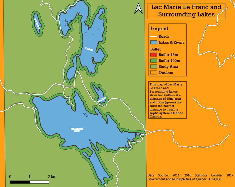
The goal for this demonstration is to find a set of lakes in Quebec cottage country where you would want to construct a cottage or house that would require a septic system. Septic systems in Quebec must have a minimum distance of 15m from the edge of a Lake, watercourse, swamp or pond. This is stated under section 7.2 of Regulation respecting wastewater disposal systems for isolated dwellings by LegisQuebec. With this information in mind, we will create two buffers. One that is 15m from the edge of the lake (assuming this is the high-water mark) and another that is 100m from the lake (which has randomly been chosen to demonstrate the capabilities of the multi-distance buffer). After both buffers have been completed, a map with proper labeling will be created as a final product.
Process
Import Data
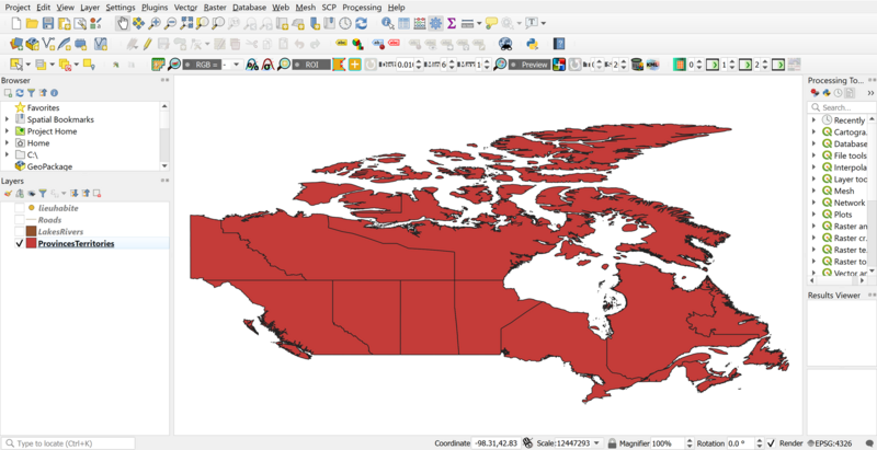
Import the data into QGIS under Layer → Add Layer → Add Vector Layer or by finding your directory under your Browser panel. Once all four layers have been loaded, re-name them as you wish for easier identification down the road. For example ghy_000c11a_e to LakesRivers.
Reproject
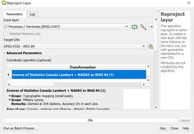
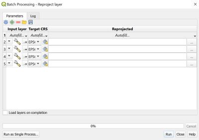
Next, we will fix the projection so that the boundaries look nicer and that the project’s units are in metres. Under the Vector tab → Data Management Tools → Reproject layer select the ‘Run as Batch Process…’ button at the bottom left of the window.
Once the new window has been opened, select Autofill → Select From Open Layers. A new window will pop up: click Select All then click OK. Set the target CRS to WGS 84 [4978].
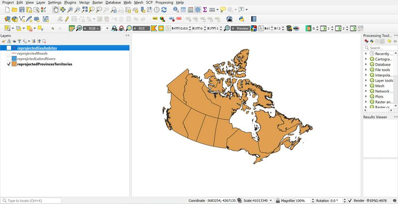
Once the CRS is set, click the three dots → name as 'reprojected' and save the files in your working directory as a shapefile. Under Autofill Settings select Fill with parameter values under Autofill mode and Input under Parameter to use. Check off the ‘load layers on completion’ box at the bottom left then click Run.
Note: It is important to make sure your new layers are created in compliance with how your operating system saves its files. i.e., no special characters or spaces etc. Additionally, you may encounter a ‘?’ beside each one of your layers indicating the layer has not been assigned a CRS. If this is the case, click on the ‘?’ and assign the CRS to the same projection as you have just performed (i.e., WGS 84 [4978]. Additionally click the CRS button at the bottom right corner of QGIS (little globe) and make sure it is set to WGS 84 [4978].
Install the Plugin
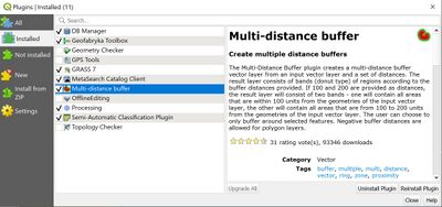
Under Plugins → Manage and Install Plugins… search for ‘Multi-distance buffer’ and click install.
Fix Invalid Geometries
In this section we will fix some invalid geometries as there are some issues with the reprojectedLakesRivers layer where the geometries are not aligned.
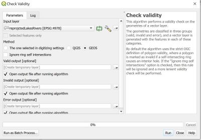
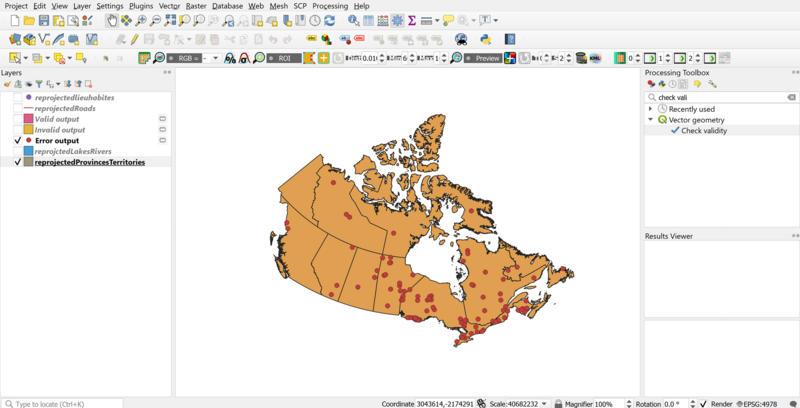
In your Processing Toolbox search for Check Validity open up the tool. Select your lakes and rivers layer under Input Layer and keep all of the original settings the same.
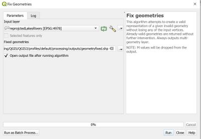
Next, under your Processing Toolbox, search for the Fix Geometries and open the tool. Select your lakes and rivers layer under Input Layer and make sure you save the file to your working directory. Click Run.
Clip
This next section will show how to clip your various layers into the designated study area you wish to do your buffer analysis. Important note: it is NOT necessary to do section 4.5.1 as it is only necessary for less powerful workstations that would have trouble loading all the lakes while panning and zooming through the map. Again, it should be noted that this demonstration works on any polygon of your choosing, therefore you do not have to select the same lakes that will be subsequently shown.
Province Clip
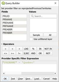
Right-click your Provinces and Territories layer and select Filter, this will open up your Query Builder.
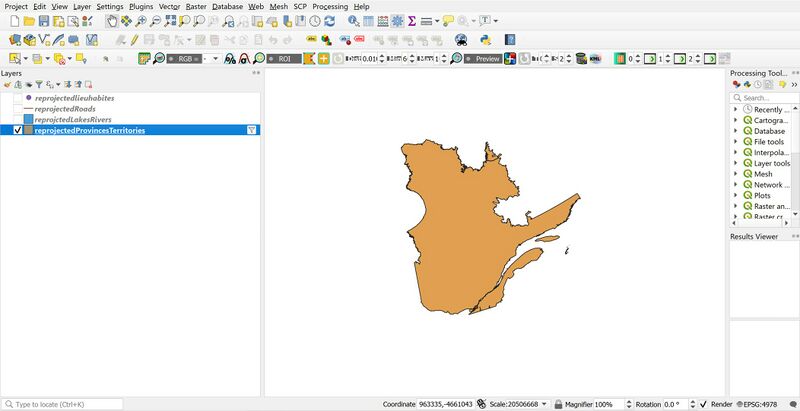
To select only the province of Quebec, in the query builder, input the following query: “PRENAME” = ‘Quebec’. Click OK. Now only the province of Quebec should be visible in your view.
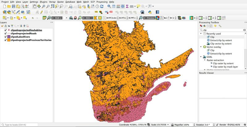
Next, we will clip all four layers to the extent of the province of Quebec. To do this, under the Processing Toolbox, search for the Clip tool, right-click and select ‘Run as Batch Process’. Under input layer, click Autofill → Select From Open Layers, a new window will pop up: click Select All then click OK. Next, make sure your overlay layer is set to your Provinces and Territories layer then click the three dots → name as 'clipped' and save the files in your working directory. Under Autofill Settings select Fill with parameter values under Autofill mode and Input under Parameter to use. Check off the ‘load layers on completion’ box at the bottom left then click Run
Study Area
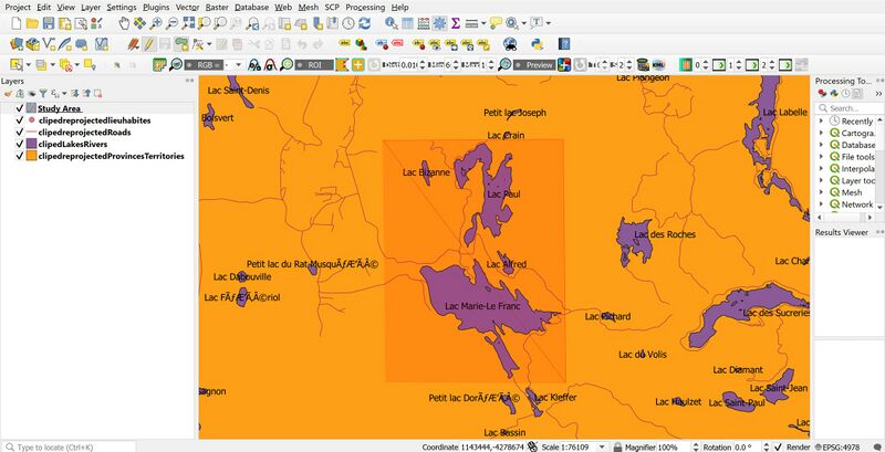
First, what we will do is create a new shapefile layer with a geometry type as a polygon. Layer → Create Layer → New Shapefile Layer. Make sure the new layer is set to the current CRS. Once you create your new layer, toggle editing by clicking the pencil icon → Create Polygon Feature then draw out your study area.
Once your study area has been created, we will now clip the four layers to the extent of the study area. To do this, under the Processing Toolbox, search for the Clip tool, right-click and select ‘Run as Batch Process’. Under input layer, click Autofill → Select From Open Layers, a new window will pop up: click Select All then click OK. Next, click the three dots → name as “extent” and save the files in your working directory. Under Autofill Settings select Fill with parameter values under Autofill mode and Input under Parameter to use. Check off the ‘load layers on completion’ box at the bottom left then click Run.
Buffer
Now that we have created our study area, it is time to use the multi-distance buffer to create our buffer distances.
Dissolve
First, we will use the dissolve function on the lakes and rivers in order to eliminate the islands on the lakes since we are only looking to build along the shoreline of the lakes. If you wanted to include the islands in your analysis, you would have to outline the islands manually and create a polygon layer for the islands themselves and use a single-sided buffer to do a similar analysis.
To use the Dissolve tool, under the Processing Toolbox, search for Dissolve and open up the tool. Select your Lakes and Rivers layer as your Input and click Run.
Multi-Distance Buffer
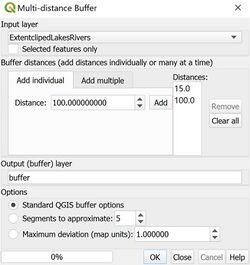
To open the multi-distance buffer, look for the red and green bean-like icon on your panel. If this cannot be found, you can find the tool under Vector → Multiple Distance Buffer. Once it has been opened, select your lakes and rivers layer as your Input layer and add two individual distances of 15 and 100. Keep the remainder of the settings the same and click OK.
You will notice now you will have two buffer distances, one at 15m and one at 100m around your lake(s). We will have to categorize these two distances, but first we will clip and create an overlay to account for roads crossing over the buffer.
Buffer Roads/Overlay
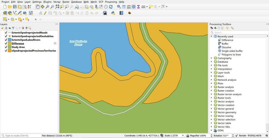
Under the Processing Toolbox, search for the Buffer tool, double-click and add the roads layer as your Input Layer. Select a distance of 10 metres and keep the rest of the settings as they were. Click Run. Next, we will create an overlay to include the new road buffer with the multi-distance buffer we executed in the previous step. Under the Processing Toolbox, search for the Difference tool and double-click. Select the Multi-distance buffer as the Input Layer and the road buffer as the Overlay layer. Keep the remainder of the settings as they were and click Run.
Categorize the New Buffer Layer
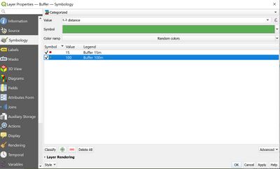
To categorize your new buffer layer, open up the Symbology tab under Layer Properties from your buffer layer. Select Categorized as your symbol, Distance as your value, then click the plus button twice to add two entries. Add values of 15 and 100 respectively and choose an appropriate colour for each entry. Once you are satisfied, click OK.
