Beginner's Tutorial to GRASS GIS in Python
Introduction & Purpose
Throughout my brief years of study at Carleton University in the Geomatics discipline, I have noticed a shift towards a more ‘user-friendly’ focus in developing GIS tools. A great example of this initiative is the recent updates done to GRASS GIS with GRASS GIS83 improving the user GUI exceptionally with a single panel housing all the tools rather than many separate windows.
This apparent shift away from the traditional coding roots of GIS to a GUI dominant interface comes with upsides, downsides as well as an entirely new range of audience members. The focus of this tutorial is to explore the simple use of Python scripts written in Python 83 (8.3.10) using an open source IDE, in GRASS GIS83 using the pre-installed grass.script package in GRASS. The tutorial will consist of a few simple analyses using data from a few sources such as Open Ottawa and Ontario Geohub to demonstrate the capabilities of using GRASS with script rather than individual tools and the time it saves a user, especially when completing repetitive tasks.
From my personal experience the hardest part to kick-start your GIS coding experience is finding the resources and knowing where to start. This tutorial aims to fill the gaps in knowledge of a beginner GIS user looking to use code in GIS through a user friendly method available in GRASS. Therefore, the audience to this tutorial is marketed at beginner users that know the basic working principles of GIS, and are looking for a taste of scripting in there analysis process.
Software and the Environment
There are a few software downloads and installations required to follow along, as well as a few preliminary steps to setting up the environment, all of which are open source and free to use! Note that this tutorial is performed on a Windows operating system and thus will follow with Windows examples, for the most part the code in BASH for Mac or Linux is similar but feel free to reference online material to compensate!
- 1. Download a Spyder compatible version of Python
The first step is to download a Python Interpreter off of the Python website ([1]), as well as set up the directories we wish to work with. Scroll to the bottom of the Python website and, for windows users, download the 64-bit windows installer. For Mac users install the corresponding Mac installer listed in the table.
Pay close attention to the option to add Python to your system's or user PATH. This allows your computer to search python for any executable files required. In addition, note down the path to where python was installed to be sure we can select the correct interpreter in the IDE.
- 2. Download GRASS GIS
The second step to this process is locally downloading GRASS GIS from their website ([2]), and follow the installation instructions taking note of the directory you choose to save it in. In addition, upon installing GRASS you must also create a Grass database location, which is essentially a folder GRASS will look to store data in. I suggest you create this folder within the PyGIS folder in a folder named GrassData!
- 3. Creating the Virtual Environment
To complete the seemingly daunting task of creating a virtual environment we are going to make use of the python package Virtualenv. This package allows the user to create a user defined environment to keep all their code related projects organized and in check.
- First: Take the noted location of your Python installation, and open up either Bash Terminal or Windows Command Prompt and type the following code into the terminal switching the directories to the ones that correspond with your machine: cd C:\Users\colli\AppData\Local\Programs\Python\Python38\Scripts.
This line of code tells your system exactly which directory you want it to work from for the first step which is installing Virtualenv. Inside the Scripts folder is the application called pip which is Python's package installer. Once you have entered the line of code starting with cd, enter: pip install virtualenv, which will initiate the download and installation.
- Next: We are going to create our Virtual Environment with a meaningful name related to the project as well as a target directory to create our environment. To do so, enter this line of code in respect to your specific path: virtualenv C:\Users\colli\PyGIS. Note I named my virtual environment PyGIS so I know in the future that is my environment for working with GIS related data in Python!
- Moving Forward: The next step is to enter the file explorer, and within your virtual environment folder, under the Lib folder create a folder named packages. We now need to download our Integrated Development Environment called Spyder from the pip installer.
I highly recommend the Spyder IDE ([3]) as it comes equipped with a few useful tools to beginners such as a syntax dictionary/troubleshooter as well as different panels for viewing plots and other outputs. This can be particularly useful when doing higher level analysis to data that is associated with a location, such as Census data. With the plot tab you can view any graphs created or plotted, as well as any mapping products created or visualized within the IDE, but for the purpose of this tutorial we are strictly making use of GRASS GIS to exemplify the 'foundation' GIS finds in coding.
The code for the command line is: pip install spyder --target C:\Users\colli\PyGIS\Packages with of course your path reflecting your directories.
- In Continuation: We must now activate our virtual environments and subsequently launch Spyder! There are a few options to going about this task, but for me personally as a beginner using the direct cd command to launch things really gave me an idea of how a computer runs and searches for things so we will make use of that and only touch on the PATH variable.
Enter this code to manually search the virtual environment code and activate the virtual environment: cd C:\Users\colli\PyGIS\Scripts & activate.
- Finally: We will launch spyder which is stored in our packages folder under the bin sub-folder. We will access it using the cd command as always cd C:\Users\colli\PyGIS\Packages\Lib\bin & spyder.
This command should launch spyder from your virtual environment and is a relatively routine baseline standard to coding in an organized manner. Not all compupters will respond well to this, especially those in already poor conditions such as mine. If that is the case for you, you can always skip the virtual environment and either download spyder directly from their website ([4]) ([5]).
- 4. Exploring the Environment
Finally after launching Spyder we must familiarize ourselves with our workspace and ensure we switch our interpreters to the interpreter in our virtual environment!
- First: Much like before use pip to install numpy and matplotlib if they are not already installed with your python download (you can use pip to check).
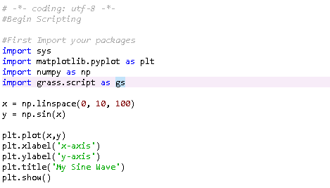
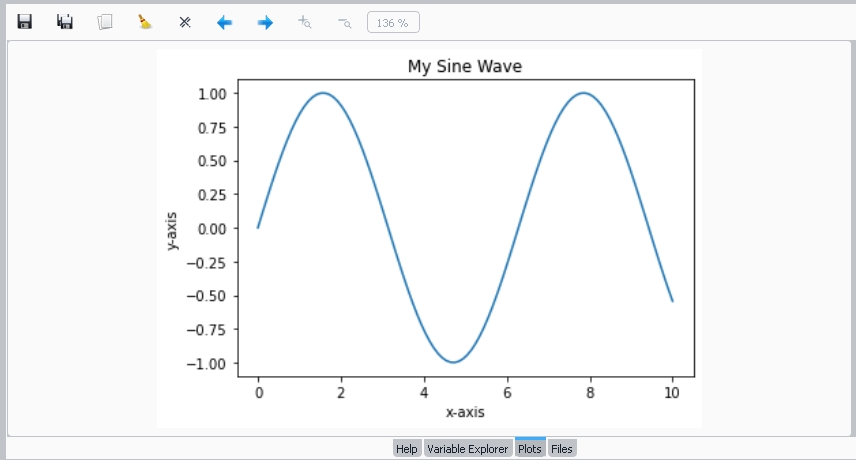
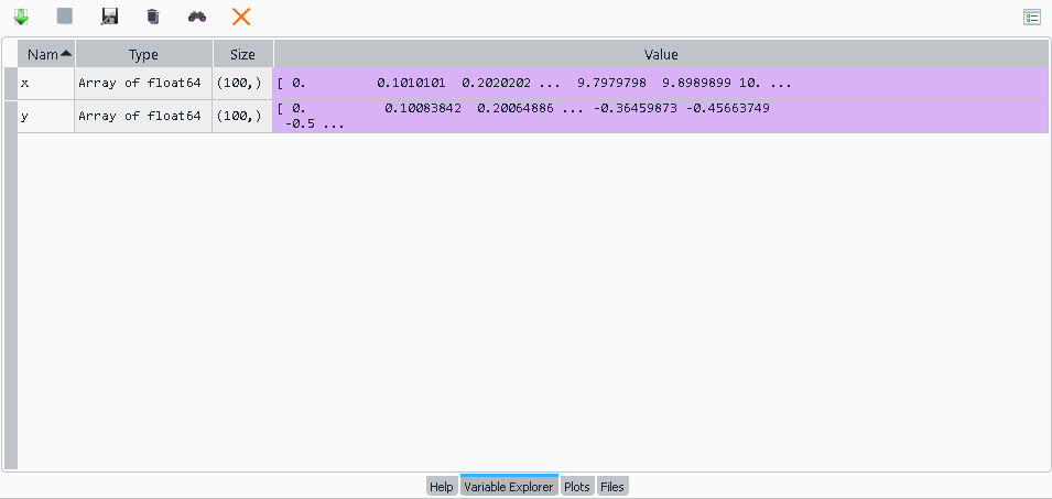
- Next: Enter this sample code to demonstrate creating a plot within Spyder, making use of the plot tab for displaying your created image, as well as the variable tab to keep track of your defined variables.
The code begins by defining the x and y variables to be used within the sine wave graph. We make use of numpy, a package that adds a lot of mathematical tools and capabilities to Python, to declare these variables and "linspace" to create an array for the x variable. We imported matplotlib as plt for simplification and use the displayed command lines to plot the declared variables, add labels and a title and then show the plot in the plot tab.
Analysis Data
- Now that we have covered a simple use of 2 Python packages, we must collect the data we intend on using in the analysis. This tutorial aims to focus on open source data and data sources making use of readily available data from two sites: USGS Earth Explorer([6]) and Open Ottawa ([7]). If you have never used Earth Explorer I have another tutorial on flood analysis mapping in GRASS that covers how to go about using and signing up for EE ([8]).
- The first data set we need is a Digital Elevation Model (DEM) which is a raster that displays the local elevation at 30 Arc-seconds. To find this dataset head over to USGS's Earth Explorer([9]), and in the Address search criteria enter Ottawa Ontario. Next, under Digital Elevation select GMTED2010 (the Global Multi-resolution Terrain Elevation Data2010 by the USGS) to search for the appropriate Tiff file. Once found select the 30-arcsecond data file which is the smallest file available. Save this file in a folder titled Data in PyGIS.
- The next dataset needed for the analysis is the Ottawa Boundary GeoJSON. One can be downloaded from the Ottawa Neighborhood Study Page in the Data catalogue on the Open Ottawa Data page provided above. Be sure to download GeoJSON format.
- Finally form the same website as the boundary file download the point file Bike repair stations and Cycling Network as shapefiles and store them within the data folder as well.
- With the data collected we can begin scripting the analysis in Spyder to launch within the GRASS GUI. There are a few advantages to doing so, mainly efficiency once the necessary skills and knowledge are present.
Sample Analysis
- Now that the data is unzipped and located in one location, we can get started with conducting a simple but meaningful analysis using GRASS GIS scripts. It may seem impractical to use Scripts at a surface level, especially when just beginning your endeavors with GIS, but it is most certainly a useful skill to have the basics of to reduce redundancy and increase efficiency especially when performing a large amount of repetitive task.
- 1. Step One: Create a Script that Imports and Clips the data.
- To create the following Script that imports the analysis data and clips it returning the raster and outline we wish to work with I referenced the GRASS GIS manual that provides full details on each function and its accompanying parameters ([10]). I make use of a few key functions within the Grass Script package all of which require gs.run_command as a precursor to execute the desired grass function.
- I use the r.import function and the v.import function to import both the raster and vector layers. The import command accepts a few parameters, namely an input parameter which is just the path to the desired file. Note you must include the file type i.e .tiff or .shp.
- After the import commands, notice I set the region to one of the imported vector layers, this is a crucial step within GRASS. Setting the region allows the software to recognize the Spatial extent, Resolution and Projection/CRS.
- Finally, I use the r.mask function to create an overlay of the DEM only where there is an intersection of the selected vector layer (Ottawa Boundary). This allows us to isolate where we want to clip on the DEM and the r.mapcalc saves it to it's own file.


