Network Analysis in Python

Introduction

Summary

This tutorial explores some basic network analysis in Python using the OSMnx and NetworkX packages.

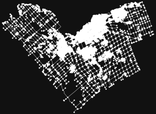
First, a road network for Ottawa, Ontario is imported from OpenStreetMap (OSM) with OSMnx. The Nominatim API is used for geocoding - no external data download required. Then, shortest path examples are shown, first distance-based, then based on travel time. The incomplete nature of OSM datasets is explored in this section. Additional features such as creating *n* number of shortest paths, comparing routes, plotting with OSMnx, and exporting a route to a shapefile are shown. Finally, a basic example of the Travelling Salesman Problem (TSP) is demonstrated.

This tutorial expects that the reader has at least a basic knowledge of Python.

Setup

Instructions for setting up a Jupyter Notebook with Anaconda and Google Colab are shown below. The only differences between the methods are found when installing the packages, exporting data, and the fact that geocoding seems to take somewhat longer with Google Colab.

Anaconda

A Jupyter Notebook of this tutorial is planned to be provided in the future.

Download Anaconda here

Setup your Conda environment with the required packages by entering the following commands into Anaconda Prompt:

Create an environment

conda create -n network_analysis

Activate the environment

conda activate network_analysis

Install required packages

conda install -c conda-forge jupyter notebook osmnx

NetworkX, Geopandas, Pandas, and Numpy are all dependencies of OSMnx and will also be installed. Enter "y" for yes if prompted

Google Colab

Add the following to the start of your notebook:

!pip install osmnx

NetworkX, Geopandas, Pandas, and Numpy are all dependencies of OSMnx and will also be installed.

Import Required Packages

import pandas as pd
import numpy as np
import geopandas as gpd
import networkx 
import osmnx

Quick Review of Networks and Graphs

Basics

Networks are abstract structures that represent relationships between objects. Their applications vary widely, from social network analysis to neural networks in the brain, transportation planning, and stream network analysis. Graphs are used to represent and analyze networks mathematically.

Graphs are composed of two parts:

Nodes -> things or objects

road intersections

Edges -> links or connections between nodes

road segments

Edges can be directed or undirected (single or bi-directional).

Directed edges are useful for analysing stream networks, or in this tutorial for highways and one-way streets.

The study of the arrangement of nodes and edges in relation to each other, as well as in physical space, is known as Topology.

For more information, check out the Open Geomatics Textbook here.

Data Structure

Graphs, DiGraphs, MultiGraphs, and MultiDiGraphs are the data structures used by packages like OSMnx and Networkx.

Graphs and DiGraphs represent simple undirected and directed graphs respectively. "Multi-" means that multiple parallel edges are allowed, like multiple lanes on a highway.

Note: "parallel" in graph theory means that two edges connect Node A to Node B. This does not apply to bi-directional streets, since one connects A to B, and the other connects B to A, even though we would consider those lanes to be geometrically parallel.

The data imported in this tutorial is by default a MultiDiGraph, which suits the purposes of this tutorial.

For more information on the different graph data types, see the NetworkX documentation here.

Indexing for Edges and Nodes

Throughout this tutorial, we will often be converting from MultiDiGraph to GeoDataFrame to explore the data. OSMnx converts a MultiDiGraph into separate GeoDataFrames for nodes and edges. Nodes use their OSM ID as their index, while edges use three indexes. The first ("u") and second ("v") show the OSM ID of the source and target nodes respectively, while the third index ("key") is used to differentiate multiple parallel edges. This tutorial does not use multiple parallel edges, so this key will always be 0.

Importing OSM Data

To explore some of the network analysis options in Python, this tutorial will use the road network of Ottawa, Ontario. This can easily be acquired using the OSMnx package, which uses Overpass API. The graph_from_place() function geocodes the area of interest (AOI) query and filters the network to the City of Ottawa's boundaries, while graph_from_polygon works with a custom polygon.

For additional information, check out the OSMnx documentation here and the example gallery here.

# create query for Smiths Falls
AOI = "Ottawa, Ontario, Canada"

# retrieve road network -> this may take some time
graph = osmnx.graph_from_place(
    AOI,
    network_type="drive" # this selects roads only. Other network options include "bike" and "walk".
)

# visualise the road network
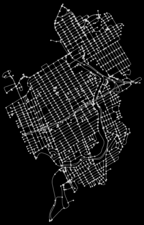
figure, ax = osmnx.plot_graph(graph)

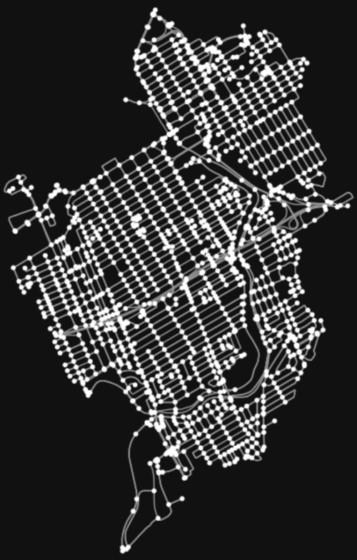
Let's pick a smaller area that is easier to visualise. A geojson boundary is provided below, but can be replaced with any custom polygon.

# Downtown boundary -> this can be replaced with any geodataframe
ott_boundary_geojson = {
"type": "FeatureCollection",
"name": "ott_boundary",
"crs": { "type": "name", "properties": { "name": "urn:ogc:def:crs:OGC:1.3:CRS84" } },
"features": [
{ "type": "Feature", "properties": { "id": 1 }, "geometry": { "type": "MultiPolygon", "coordinates": [ [ [ 
    [ -75.700646544981723, 45.442406206090276 ], [ -75.692602224956474, 45.439061352815521 ], [ -75.690143080492803, 45.436977332083586 ], 
    [ -75.686975368980271, 45.436893971254314 ], [ -75.684016059540923, 45.438561187839852 ], [ -75.679535414967276, 45.437998502242237 ], 
    [ -75.671449414527402, 45.433851300985694 ], [ -75.67046992478339, 45.42670310987517 ], [ -75.668531785502708, 45.424410687070051 ], 
    [ -75.667531455551384, 45.42140969721607 ], [ -75.663592656368039, 45.418596269227969 ], [ -75.663092491392362, 45.415928722691106 ], 
    [ -75.664426264660804, 45.414970073154414 ], [ -75.668406744258789, 45.414365707142153 ], [ -75.670657486649262, 45.413282016361556 ], 
    [ -75.672199661990902, 45.412219165788272 ], [ -75.673095790905634, 45.410072624434378 ], [ -75.668740187575892, 45.404154005555696 ], 
    [ -75.669865558771136, 45.400173525957719 ], [ -75.672783187795829, 45.397672701079401 ], [ -75.674429564174062, 45.3940048245912 ], 
    [ -75.678014079832991, 45.389128216078483 ], [ -75.689069809815834, 45.383136656474207 ], [ -75.695373972529922, 45.381729942480156 ], 
    [ -75.700063019176767, 45.378676852107873 ], [ -75.702199140426984, 45.378176687132189 ], [ -75.701886537317193, 45.381261037815442 ], 
    [ -75.700094279487729, 45.383803543108399 ], [ -75.700531923841439, 45.387554780425873 ], [ -75.70151141358545, 45.392181306450752 ], 
    [ -75.708805486147227, 45.396057585012137 ], [ -75.713369491550125, 45.403497539025139 ], [ -75.723758334898761, 45.410385227544161 ], 
    [ -75.725748574697747, 45.418075264044965 ], [ -75.70428316115887, 45.425369336606728 ], [ -75.700646544981723, 45.442406206090276 ] 
] ] ] } }
]
}

AOI = gpd.GeoDataFrame.from_features(ott_boundary_geojson["features"], crs="EPSG:4326")

# retrieve road network -> this may take some time
graph = osmnx.graph_from_polygon(
    AOI.geometry.iloc[0],
    network_type="drive" # this selects roads only. Other network options include "bike" and "walk".
)

# visualise the road network
figure, ax = osmnx.plot_graph(graph)

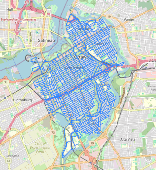
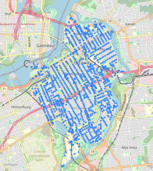
Let's examine the network with a basemap. We can do this by extracting the nodes and edges of the graph as geodataframes and using the .explore() method from GeoPandas.

# create geodataframes
nodes, edges = osmnx.graph_to_gdfs(graph)

# view edges with basemap
edges.explore()

# view nodes with basemap
nodes.explore()

This looks good. Now let's customize some of the plotting parameters.

The configuration below can be easily applied as a base for any OSMnx plot we create later on.

Feel free to experiment!

Read the OSMnx documentation for further customization options.

# plot settings -> to be used as a base for most plots later on
pgr_args = {
    "figsize": (8, 10),           # figure size (width, height)
    "bgcolor": "black",          # background colour
    "node_color": "black",       # colour(s) of the nodes
    "node_size": 5,              # size(s) of the nodes
    "node_alpha": 1,             # opacity of the nodes
    "node_edgecolor": "white",   # colour(s) of the node borders
    #"node_zorder" : 0           # this will plot nodes under the edges
    "edge_color": "grey",        # colour(s) of the edges
    "edge_linewidth": 1,         # line width(s) of the edges
    "edge_alpha": 1,             # opacity of the edges
}

# plot graph with new settings
fig, ax = osmnx.plot_graph(graph, **pgr_args)

Simple Routing: Shortest Path

1. Distance-Based

2. Time-Based

3. Route Comparison