Network Analysis: Finding shortest path in QGIS
Contents
Introduction
Calculating the shortest distance between two points is a commonly cited use for GIS. QGIS (Quantum GIS), an open source software ships with this tool, but it’s not visible by default. In this tutorial we will show you what you need to get started.
Data
The data are provided by City of Ottawa Open Data Catalog. It was used a polyline shapefile of Ottawa roads and a point shapefile of museums. This project is focused mostly in downtown Ottawa area. The shapefiles should be located in the same folder, in which we are going to work on.
Acquiring QGIS (version 2.6)

You may go to this link : QGIS(v.2.6) in order to download the QGIS version that is suitable to the operating system you are working on.
- After the software is downloaded and ready to execute, we double click the QGIS shortcut icon on Desktop. The GQIS window opens.
Set up the Environment
The type of the data that we are going to work are vector data. The first step is importing the shapefiles in the QGIS environment.
Add vector data
In Layer menu, select Add layer and choose Add Vector Layer. Another option is click the Add Vector Layer button of the toolbar
Projection
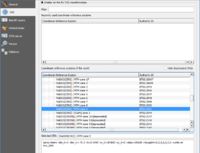
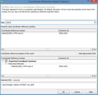
All the layers were projected under EPSG:2951 - NAD83(CSRS) / MTM zone 9 projection. Right click on the layer, select Project Properties, from which we choose CRS. Then we select the appropriate projection for our case. This process is done for all the layers that we are working with.
Area of Ineterest (AOI)
The project is focused on determining the shortest path between Museum of Nature and Museum of War in downtown Ottawa area. That's why it is important to get rid of abundant data. In this case we had to create an AOI.
- In Layer menu, choose Create Layer, then New Shapefile layer and the New Vector Layer window will show up. The AOI should be a polygon.
- Click the AOI layer.
- Click the Toggle on button to start editing the layer.
- Create the polygon, by clicking points on the map. On the last point of the polygon, right click so we finish creating it.
Also the AOI needs to be projected with the same projections as other layers.
- Right click on AOI layer
- Select Properties
- Choose CRS
- Filter the code 2951 in the filter tab to find faster the projection NAD83 MTM9
Clip tool
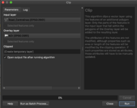
This tool is found under the Geoprocessing Tools of vector data. It is useful to clip the roads shapefile by using as clipping area the AOI.
The same steps were conducted also for the museums shapefile.
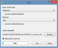
- Input vector is the layer we want to clip: Museums
- Clip layer is the AOI we just created
- Output shapefile is specified by us. it should be browsed in the same folder where other shapefiles are stored.
Symbology
It would be good to categorize the clipped roads that we got lately. We categorized them by type.
- Right click on the roads layer
- Select Properties
- Choose Style and on the very top left button select Categorized and Column: Type
- Double click on the symbols of each roads type to edit them.
Road Graph Plugin
The Road Graph Plugin is a C++ plugin for QGIS that calculates the shortest path between two points on any polyline layer and plots this path over the road network.
Main features:
   *   Calculates path, as well as length and travel time.
   *   Optimizes by length or by travel time.
   *   Exports path to a vector layer.
   *   Highlights roads directions (this is slow and used mainly for debug purposes and for the settings testing).
Activate the Tool
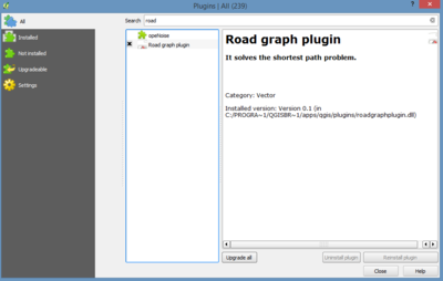
To activate the Road Graph plugin: Start the Plugin Manager by clicking on the QGIS main window’s menu item Plugins ‣ Manage Plugins. A dialog appears. Click OK on the Plugin Manager dialog.
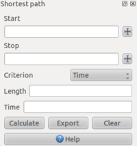
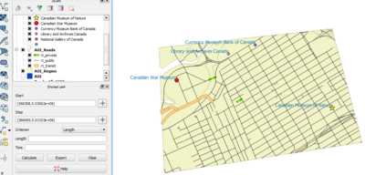
This panel will appear in your interface
If the plugin doesn't show automatically in your interface, go to View ‣ Panels and ensure that Shortest path has a check mark next to it.
Configure the Tool
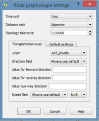
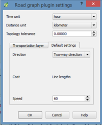
Time Unit and Distance Unit we leave as default in hour and kilometer. Topology tolerance: In case if there is a gap between two lines to treat them as continuous, the topology tolerance may be applied, for example 10m. In our case we left as default 0. On the Transportation Layer, we choose the layer of the roads. In this case the clipped roads. For the direction field we leave as default. In other cases, while in the attribute table we might have a direction field, we might use the value of this field for direction. For this project we don't have any data for the direction. We keep the speed limit as default. And we choose the speed limit value under the Default Settings tab. For this example the speed was chosen 60 km/h as shown in Figure below.
Use the Tool
Suppose we want to calculate the distance in length from Canadian Museum of Nature to Canadian War Museum. In the plugin panel, click on the Capture Point button next to the Start field:
- Click point that represent Canadian Museum of Nature as start point.
- Use the Capture Point button next to the Stop field and capture the point of Canadian War Museum.
- Click on the Calculate button to see the solution:
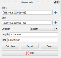
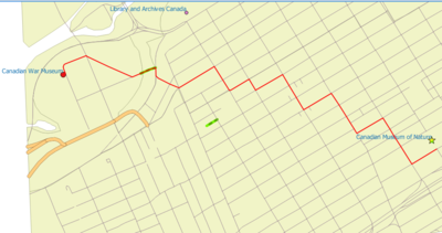
The result for the shortest path is shown below. This is a simple case, where the speed mode is the same for all the streets, 60 km/h.
Using Criteria
What happens when different streets in the network road have different speed limits?
The idea is to set different speed limits for some of the selected streets by us. In this case we had to add a new field in the roads layer and call it Speed.
Create New Field
- Right click on the roads layer.
- Call this new column SPEED, and give it the type Whole number (integer) with a width of 3.
Queries
Now we had to run some selection attribute query over the road layer, in order to specify the speed limit 50 km/h for the private roads,60 for public roads with the name BRONSON, 45 km/h for the public roads with name GLOUCSTER and 30 km/h for the rest of the roads.
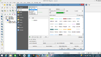
- On the bottom left corner of the Attribute Table, there is a Show All Features button. Click on the arrow and select Column Filter *Then choose for example TYPE, because we want to select the private roads.
- As you write rt_private automatically will appear the Advanced Filter expression.
- Select private roads and assign the speed limit 50 by using Advanced Filter expression
- Select public roads with name BRONSON and assign the speed limit 60 by using Advanced Filter expression
- Select public roads with name GLOUCESTER and assign the speed limit 45 by using Advanced Filter expression
- Select the rest of the public roads and assign the speed limit 30 by using Advanced Filter expression
After assigning the speed limits for each selection we save the edits by clicking the save button and then click the toggle button again to turn off the edit mode.
Use the tool after criteria is done
- Check the Vector ‣ Road graph ‣ Road graph settings to ensure that it’s set up as explained previously in this tutorial, but with the Speed value set to the SPEED field you just created.
- In the Shortest path panel, click the Start point button.
- Set the starting point to where the point of Museum of Nature is located.
- Set the end point to the Museum of War location.
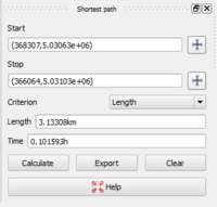
- In the Criterion drop-down list in the Shortest path panel, select Length.
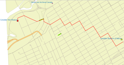
- Click Calculate. The route will be calculated for the shortest distance:
Notice the values of Length and Time in the Shortest Path panel.
And this is the result graphically of the shortest path in distance
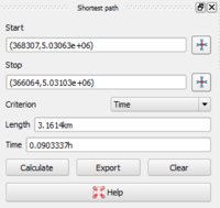
- Set the Criterion to Time.
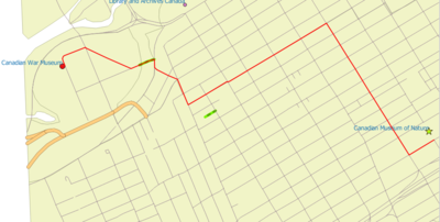
- Click Calculate again. The route will be calculated for the shortest time:
- You can switch back and forth between these criteria, recalculating each time, and note the changes in the Length and Time taken.
The Shortest Time path result as shown below
- The last operation is to export the output as a shapefile, by clicking the Export button on the Shortest path panel.
Conclusion
Road graph plugin used in QGIS, helped defining the shortest and the fastest way to get from Canadian Museum of Nature to Canadian Museum of War, based on the cost length. It is important to verify the settings. You could verify from the output that if the speed limit is the same in all the roads, the shortest distance would be the same route for the length and time cost. While if we apply different speed limits for different segments of roads, than there is difference between the shortest path way for length cost, compare to shortest path way for time cost.
Future work
Future work might be creating Drive Time isochrones in QGIS. Site analyses can benefit greatly from using “drive-time” isochrones to define the study area. In ArcGIS this is called Sercive Area. It might be helpful (pgRouting) open source software to create the nodes network, which each of them would define a start and an end point for different segments that create the network. This is benefical for airports. If the location of airports are consider to be the nodes of the network, then a routable network graph with adequate weights would be created by pgRouting. The first step is to find the closest network node to every airport. The next one is to calculate drive times between network nodes and “airport nodes”. The resulting point layer than can be imported into QGIS. Using TIN interpolation (from Interpolation plugin), we can calculate a continuous cost surface. And Contour function (from GDALTools) yields drive time isochrones. Based on this analysis, it is possible to determine how many inhabitants live within one hour driving distance from an airport or how many people have to drive longer than e.g. ninety minutes to reach any airport.
References
- QGIS. (2014) Road Graph plugin. Retrieved Dec 15, 2014 http://docs.qgis.org/2.6/en/docs/user_manual/plugins/plugins_road_graph.html
- ArcGIS. (2014) Sercive Area Analysis. Retrieved Dec 15, 2014 http://help.arcgis.com/en/arcgisdesktop/10.0/help/index.html#//004700000048000000
- QGIS. (2014). QGIS: A free and Open Source Geographic Information System. Retrieved December 15, 2014 from http://www.qgis.org/en/site/index.html
- QGIS. (2014) Download QGIS for your Platform. Retrieved on December 15, 2014 from http://www.qgis.org/en/site/forusers/download.html
- QGIS. Blog (2014) Retrieved on December 16, 2014 http://planet.qgis.org/planet/tag/drive%20time%20isochrones/
- Roadways (2013). City of Ottawa Open Data Catalog Retrieved on December 15, 2014 http://data.ottawa.ca/dataset/roadways
