Data Extraction and Analysis Using Free and Available Software

Introduction and Purpose

The use and manipulation of raster data is an integral part of GIS, and can play an important role within urban planning. This tutorial will demonstrate how to extract and utilize available raster data for all areas where data may not already be available (eg: rural towns). This is particularly important if you are working on a project where the information has not yet been created, or you want to double check questionable data. The tutorial will demonstrate the capabilities of open source software, and the many possibilities from the perspective of an urban planner, who may not have access to expensive subscriptions or information in certain areas or regions. You will be introduced to data extraction and analysis within the realm of planning, wherein it falls to the planner to find the best site for a home in a crowded area -- when this has been located, it's important to check if the area is on a flood plain or low lying area as the chosen site is surrounded by water (the Ottawa River and Rideau Canal).

Software

The links and descriptions for the software used for this tutorial are as follows:

QGIS

Version 3.4.2 'Madeira'

QGIS is a free and open source GIS. This means that is a powerful tool that allows for the manipulation and analysis of spatial data, and can be downloaded by everyone.

Download available here.

Ensure that version 3.4.3, 64bit is downloaded.

Google Earth Pro

Software by Google that allows geospatial data to be extracted and manipulated.

Available for download here.

Google Sheets or Microsoft Excel

Both Google and Microsoft have excellent software for spreadsheets. While Google Sheets is free, the majority of people have access to Microsoft Excel. Google Sheets was used for this tutorial, as all people will have access to this.

1. Google Sheets is available here. Google account is required (free), and there is no download necessary.

2. Microsoft Office is available here. Must be a student at Carleton University to qualify. If you do not have access this is not a problem, as Sheets functions very similarly.

TCX Converter

Free conversion software that allows for the rendering of altitude data from Google Earth data (.kml). This allows us to create a point cloud within QGIS.

Download TCX converter here.

Getting Started and Setup

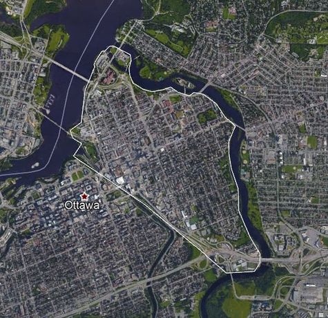
To begin, you must ensure that all software is downloaded and functional. Try running everything at least once before continuing. Once this is done, open up Google Earth Pro and locate Ottawa, or the area you would like to work with. The tutorial will be completed in the Lowertown/Sandy Hill neighbourhoods of Ottawa, found at the coordinates: 45°25'45.88"N, 75°41'7.40"W. This can be copied and pasted into the Google Earth search bar, and will put you between the two neighborhoods. Your extent should be similar to what is pictured below.

Once your study area has been located (again, it does not have to be the same as below) we will begin to use the tools within Google Earth Pro to create our study area. You'll want to navigate to Add Path in the Google Earth toolbar, pictured below.

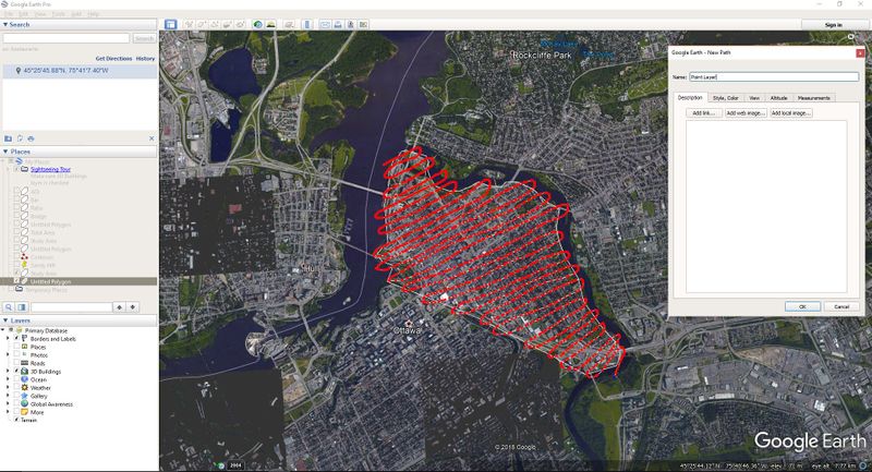
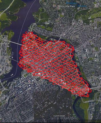
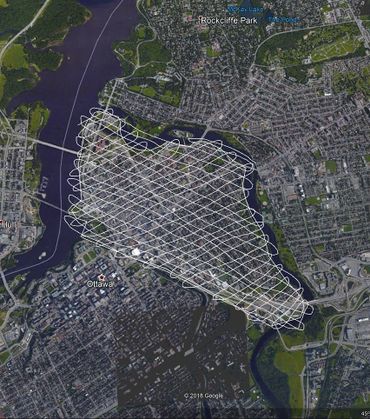
At this point you will see the window for Add Path. You can provide a name to the layer, but this is not necessary. Begin to create a thatch pattern of points across the study area by holding down the left-mouse button, similar to what you see below. The closer you get the more precise the interpolation will be (to be completed at a later step). This step takes some time, but provides the necessary data for the creation of a raster layer in QGIS. When all your points have been laid out, navigate to Altitude, and ensure Clamped to Ground is selected. When this is done, hit Ok.

• 

  Part 1 of extracting the points/elevation data. Create a series of points over the study area where the elevation will be extracted. The more points the better, but no need to go crazy here.
• 

  Part 2 of the extraction process. Create a sort of thatch by going across the area once more.
• 

  Part 3 of the process. This is similar to what your final outlook should look like. Be sure to go slightly over your study area to encapture the surrounding landscape.

At this point you will have your points and area selected for extraction. Follow these steps:

• Right-click on your point layer.
• Save Place As -> .kml
• Name the file whatever you want (eg: Point Data), and ensure you save it to your working folder.

Conversion

Now that we have our points, these need to be ran through the conversion software in order to extract the altitude data from the Google Earth .kml, and then convert to a .csv file. Open TCX Convert, which was downloaded in section the earlier section, titled Software. If it is not downloaded, do so now as it is necessary to complete this tutorial.

• 
• 

• In the top right corner of the tool, change the language to English, or your preferred language if it is not already set.
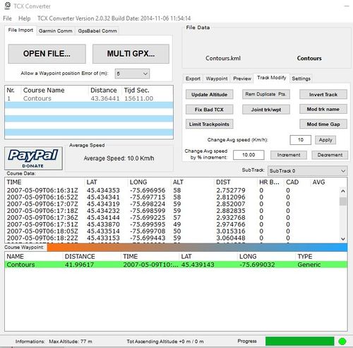
• Open File -> your point file (.kml)
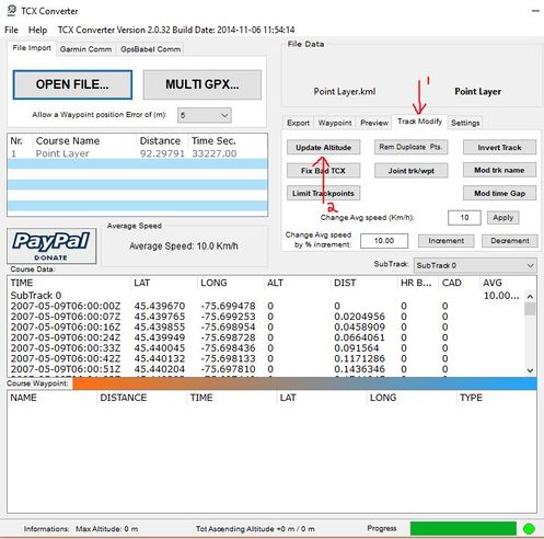
• You will notice the altitude column is 0 at this point.
• Navigate to Track Modify in the window near the top right, and then Update Altitude, and click Yes (See the image below).
• Once the progress bar has completed, navigate to Export, found in the same area as Track Modify.
• Export the file as .csv to the same folder as your other data.

The next step will be to import this .csv file into Google Sheets or Microsoft Excel -> Sheets will be explained here due it being free and accessible, as well as having slight more steps to Excel.

Spreadsheets

Open your browser and click here to head to Google Sheets. Once there, open a new sheet and navigate to:

• File -> Import -> Upload -> Select a file from your computer
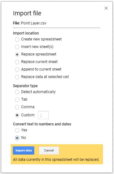
• Select the 'Point Data' file, and match the image below (ensure you do not forget the semicolon for the separator type):

This will bring the .csv into Sheets, and allows for the irrelevant data to be deleted, so it can be exported once more.

• Delete all columns aside from LAT, LONG, and ALT
• File -> Download as -> Comma separated values (.csv). When saving it, ensure that you change the name slightly so you import the correct file in the next step.

Note: If using Excel, this can all be done by simply opening the .csv and deleting the required columns. Without Excel, this is where Sheets is useful as the .csv will appear as plain text instead.

QGIS

Quick Map Services

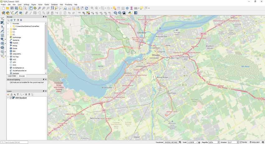
When your file has been exported as a .csv, it's ready to be brought into QGIS. Before that however, a basemap will be brought in using QuickMapServices, a plugin that simply allows for a quick basemap to be imported, such as OpenStreetMap, a highly detailed basemap that is continuously updated.

• Open up QGIS.
• Navigate to the menu toolbar at the top of QGIS
• Plugins > Manage and Install Plugins > All Plugins
• Enter QuickMapServices into the search bar, and then Install Plugin

This will download the plugin and create the following on the vector toolbar (the second one):

• Click on the icon outlined in red, which will open up the QuickMapServices plugin.
• OSM > OSM Standard

This will create the layer OSM Standard in the layers tab.

Creating Raster Data

Now the raster data can be created. Begin by navigating to the Manage Layers Toolbar, and to the icon displayed below:

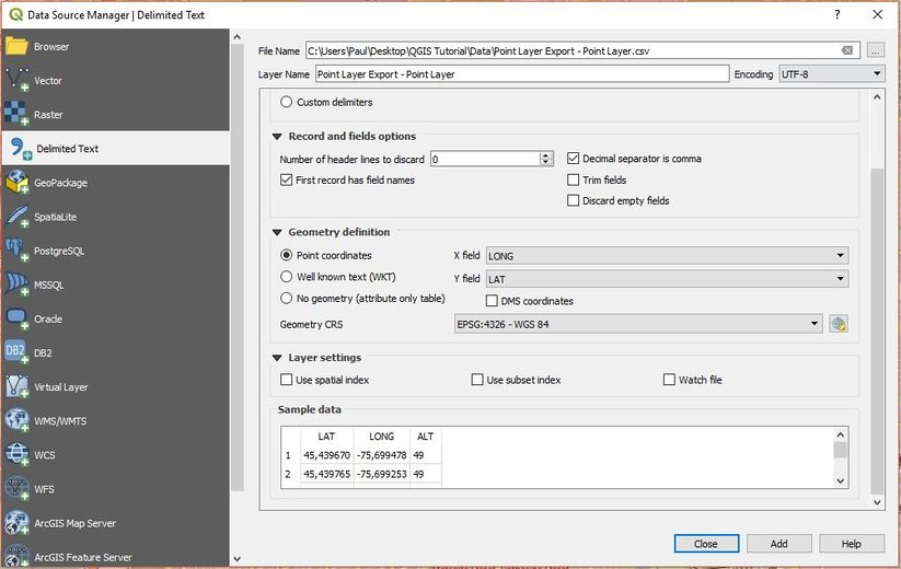
This allows for the import of the .csv into QGIS, where it can be used to create a DEM or other raster data. It is important at this stage to ensure that all selections made below are the same as what is listed/seen in the image below. 'Select:'

1. Delimited Text tool > Select the file using the three dots to the right of File Name.
2. Under File Format select CSV
3. Ensure 0 fields are discarded, and the "First Record has field names" box is checked. This maintains the column headers, and Decimal separator is comma is checked.
4. The Geometry Definition settings are very important, so check that Point Coordinates is selected.
5. After this, ensure the following is set: X == LONG, Y == LAT and Geometry CRS == EPSG:4326 - WGS 84, or the projection you have decided to use based on your selected area.

When your Delimited Text window looks the same as the image below, and the Sample Data is the same then click Add and the point layer will be created.

• 
• 

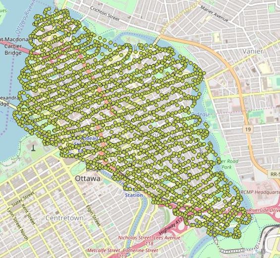
At this point you will have a series of points within QGIS that have the atrributes of Longitude, Latitude, and Altitude. This can be used to create Raster data using interpolation methods, allowing you (the user) to analyze/extrapolate a large amount of data. We now have all of the necessary information extracted, converted and imported into QGIS.

Interpolation

The processing toolbox will be used in order to turn the point/elevation data into a DEM.

Navigate to the top of the QGIS window, and select:

1. Processing > Toolbox - This brings up the processing toolbox, wherein the necessary tools can be located.
2. SAGA > Raster Creation Tools > Natural Neighbour

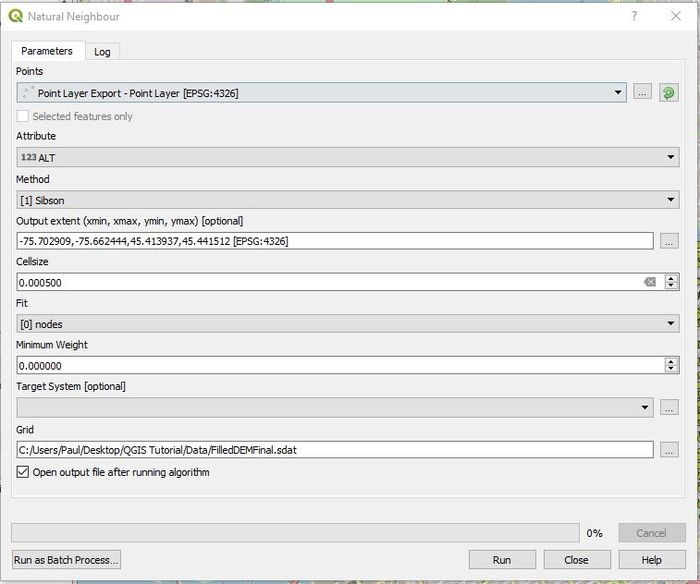
This is a form of interpolation that will benefit from a denser cluster of points. To create a natural neighbour interpolation, fill in the following parameters:

1. Select the point layer imported in the previous step using Browse.
2. Under the Attribute field, select the Altitude (ALT).
3. For the Method, select Sibson.
4. Output Extent > Use Layer/Canvas Extent > Select the point layer. This will fill in the extent to stop at the boundary of the point layer, and will extend to the furthest points around the perimeter.
5. Cellsize == 0.0005
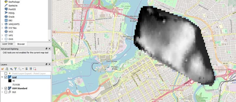
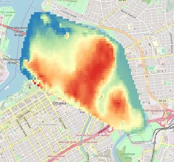
6. Under Grid, create a new save of the interpolation file, and then 'Run Natural Neighbour - See below for the outputs
   1. Right click on the layer 'Grid' > Properties > Render type == Singleband Pseudocolor.
   2. Rick click on the colour ramp (the bar and not the text), and invert it, providing a blue (low) to red (high), and demonstrating the elevation differences.

• 

  Part 1 This is the output of the Nearest Neighbour interpolation method once it has completed.
• 

  Part 2 The grid was re-symbolized to demonstrate a more dramatic change in elevation that is easier to interpret.