RQGIS, Utilizing Rstudio as an alternative GIS
Contents
Introduction
This tutorial is meant to demonstrate how to utilize RQGIS as a method of processing and analyzing spatial data. You will learn how to set up an environment within RStudio to utilize RStudio as a GIS application. Additionally, you will learn how to make use of various QGIS, SAGA and GRASS functions within RStudio by accessing their functions through the R coding language.By the end of this tutorial the user should have a basic understanding of how to utilize RStudio, and will have gained the fundamentals necessary to explore and utilize QGIS functions within RStudio.
RStudio and RQGIS
RStudio
RStudio is an open source IDE that utilizes the programing language “R”. Due to the nature of open source software, a wealth of packages have been developed for the “R” language(RQGIS included). This allow users to perform various types of statistical analysis, modeling and geospatial processes within RStudio.
RQGIS
RQGIS acts a bridge package between the functionality of QGIS and the IDE of RStudio. By installing this package, the user can access the geospatial processing functions found within QGIS from within RStudio. This allows for the user to utilize R as a geoprocessing workspace to modify and create new datasets.
Installation guides
QGIS
We start by creating a fresh install of QGIS in order to download the functions that we will be exploring in this tutorial. QGIS can be installed from https://www.qgis.org/en/site/forusers/download.html, for the purposes of this tutorial we will be installing the 64-bit version.
- After downloading the installer, open it, select Advanced install then click next
- We will be installing QGIS into the default root directory so click next to continue through the installer
- Next select install from internet and then click next
- A default directory will be created for temporary files, you can create a custom directory for these temporary files or use the default one
- Select direct connection and click next
- Select the host http://download.osgeo.org which will act as the provider for the download
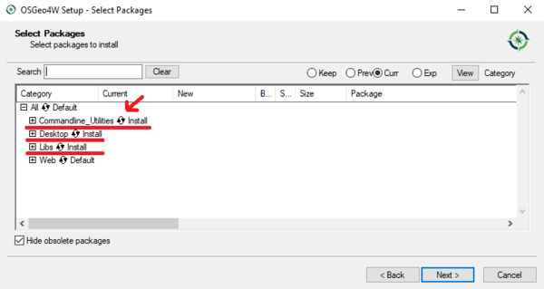
- Next click the circle to select install for: commandline_Utilities, Desktop, and Libs
R and RStudio
In order to utilize RStudio we first need to download R. This can be downloaded from https://cran.r-project.org/bin/windows/base/. For this installer we will be accepting all of the default paths and options.
Now we can download RStudio, similar to R we will be utilizing all default paths and options. RStudio can be downloaded from https://www.rstudio.com/products/rstudio/download/#download.
RStudio and RQGIS setup
Now that we have all of the software that we need we can proceed with setting up RQGIS within RStudio. In order to run QGIS functions within RStudio we will need to download and unpack some packages which allow for the manipulation of spatial data. After installing these packages within the workspace we will link our workspace with the root directory of QGIS in order to gain access to its host of functions and algorithms.
Install Packages
Start by opening up RStudio and creating a new ‘’’R script’’’ file (file->new file->R script). Within this new script we will be downloading and installing some packages that allow us to manipulate raster and spatial data within RStudio. Start by adding this code to your script and running it.
#Install packages
install.packages("sp")
install.packages("RQGIS")
install.packages("rgeos")
install.packages("raster")
install.packages("rgdal")
#Attach packages to workspace
library("sp")
library("RQGIS")
library("rgeos")
library("raster")
library("rgdal")
- sp: provides functions for plotting spatial data
- RQGIS: Creates a link between the IDE (RStudio) and functions found within QGIS
- rgeos: allows for the manipulation of vector data
- raster: Provides the user to read, write and manipulate raster images within RStudio
- rgdal: Provides the user to read, write and manipulate shapefiles within RStudio
Set workspace environment
Now that we have installed all the necessary packages we have to link the directory of the QGIS applications to our current RStudio workspace. This is achieved by utilizing the set_env() function.
#Links QGIS paths to the current RStudio workspace
set_env()
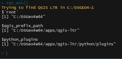
Try adding this line to your script,after running this line the console should provide path names similar to this example.
Now you have full access to all of the geoprocessing functions found within your copy of QGIS Desktop. Within this workspace you will be able to call these functions to manipulate and display spatial data.
Data Acquisition
In this tutorial we will make use of datasets that are accessible within RStudio, to demonstrate the use of various geoprocessing functions. In order to access these datasets you use the data() function which provides the user with a list of all available datasets preloaded within RStudio. Additionally the getData() function allows the user to download geographic data for specific countries around the world.
Working Directory
First we will create a folder within your main directory in order to store all of the outputs that we create within this tutorial. This folder will be placed in the first branch of your C: drive, if your computer's IOS is located on a different drive (such as a D: drive) you will have to modify the drive name within the code to match your computer's hard drive.
#Create a working directory for this tutorial
mainDir <- "C:/"
subDir <- "tutorial"
if (file.exists(subDir)){
  setwd(file.path(mainDir, subDir))
} else {
  dir.create(file.path(mainDir, subDir))
  setwd(file.path(mainDir, subDir))
}
Importing Data
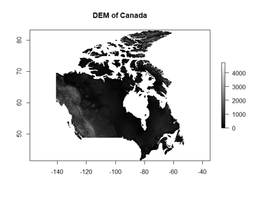
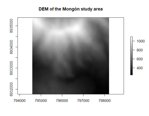
Next we will import the datasets that we will be using in this tutorial into our workspace and display them within the RStudio plot frame. We will be downloading a DEM of Canada as well as a preloaded DEM of Mt. Mongón which is located in Peru.
#Digital elevation model (DEM) of the Mongón study area
data(dem)
dem_mongon<-dem
plot(dem_mongon, col=grey(0:100/100), main='DEM of the Mongón study area')
#Digital elevation model (DEM) of Canada
canada_dem<-getData('alt', country='CAN', mask=TRUE)
plot(canada_dem, col=grey(0:100/100), main='DEM of Canada')
After running this code you will notice that the DEM's are displayed in the lower right plot window. The outputs should look like this:
.
QGIS Functions
In order to utilize QGIS functions within RStudio, we first have to learn how to find the functions we want to use with their respective syntax, as well as learn what parameters we will be working with for each function. In order to do this we will be making use of the find_algorithms() function and get_usage() function. The find_algorithms() function allows the user to enter a keyword for the function they are interested in using, and provides the user with a list of available functions that pertain to that keyword. After selecting the function that we are interested in using we can use the get_usage() function to display the parameters that the function requires as inputs. As an example we will use the find_algorithms() to search for a clipping function.
#Searches for functions which contain the keyword 'clip'
find_algorithms(search_term = 'clip')
After running this line you will see a list of 11 clipping tools that have been displayed in the console.
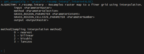
Lets select the first one qgis:clip and determine which parameters we will need to be able to make use of this function in RStudio. To do this we will use the get_usage() function. In order to use this function we need to use the full name of clip which is qgis:clip. Additionally, by setting intern=FALSE we can display the parameters in a list.
#Provides the user with information regarding the parameters of a function
get_usage(alg = "qgis:clip",intern=FALSE)
When running this line of code you will see a list of the functions parameters appear in the console. This provides you with information regarding the type of input required for each parameter and provides the user with a legend for parameters that are normally accessed through drop down boxes.
Now that we know how to search for the functions we would like to use we can go on to utilize these functions to analyze our DEM files.
Raster to Vector
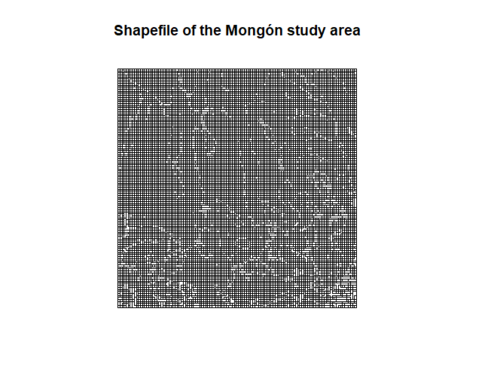
The first algorithm we will investigate is gdalogr:polygonize. This algorithm takes a raster image and converts its features into polygons. In order to use this function we will need to determine the parameters for: input, field, and output. In order to run algorithms we use the run_qgis() function. The run_qgis() function takes in the desired algorithm as well as that algorithms parameters. Here we will convert the DEM of the Mongon study area into a shapefile using the following lines of code.
#Conversion of DEM to shapefile format
run_qgis(alg = "gdalogr:polygonize", INPUT = dem_mongon, FIELD = 'values', OUTPUT = 'C://tutorial/shape_mongon')
shape_mongon <- readOGR(dsn = "C://tutorial", layer = "shape_mongon")
plot(shape_mongon)
After running this code you will see a vector interpretation of the Mongón Study area. Here is a side by side comparison between the DEM and its shapefile counterpart.
.
Clipping
Raster Clipping
In order to clip raster files we will make use of the gdalogr:cliprasterbyextent algorithm. This algorithm takes in a raster input, the desired clipping extent, output raster type and the desired output raster file. The output raster type must be the same as the input raster type, in this case our input raster is a Float32 therefore we specify the same type for our output file. Additionally, I have provided a clipping extent for the image so that we can test this algorithm.
#Clipped version of the original Canada DEM
run_qgis(alg = "gdalogr:cliprasterbyextent", INPUT = canada_dem, PROJWIN = "-121,-116,50.2,53.8",RTYPE = 5,
         OUTPUT ='C://tutorial/canada_dem_clip.tif')
canada_dem_clip<-raster('C://tutorial/canada_dem_clip.tif')
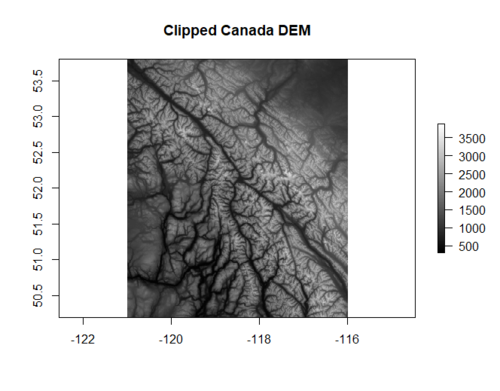
plot(canada_dem_clip,col=grey(0:100/100), main='Clipped Canada DEM')
After running this function we plot the raster image, the result should represent the western section of Canada that we specified in the algorithm.
Vector clipping
In order to clip the Vector shapefile of the Mongol study area that we created we will use the gdalogr:clipvectorsbyextent algorithm. This algorithm takes the shapefile as an input, a specified clipping extent, and a specified output for the result. Try running the code provided below.
#Take an input shapefile and clip it to the specified extent
run_qgis(alg = "gdalogr:clipvectorsbyextent", INPUT_LAYER = shape, CLIP_EXTENT = '795592,797004,8933001,8934710', OUTPUT_LAYER = 'C://tutorial/vectclip')
clipped_vect <- readOGR(dsn = "C://tutorial", layer = "vectclip")
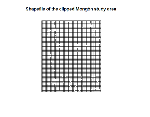
plot(clipped_vect,main='Shapefile of the clipped Mongón study area')
The result of the shapefile clip should resemble the image seen below.
Laplacian Filter
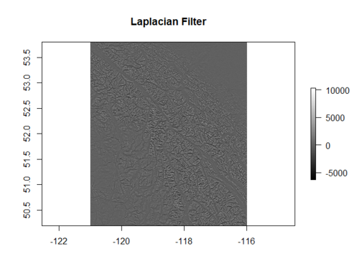
In this example we will utilize a Laplacian filter on the clipped version of the Canadian DEM. The Laplacian filter will be used to highlight the edges of the mountain range and gullies. To utilize a Laplacian filter within RStudio we will use the SAGA function found within QGIS, saga:laplacianfilter. In order to use the Laplacian filter we need an input raster, kernel method, Radius, and sampling method. The code to run this filter on the clipped version of the Canadian DEM is provided below.
#Creates a new raster image depicting the filtered Canadian DEM
run_qgis(alg = "saga:laplacianfilter", INPUT = canada_dem_clip, METHOD = 2, MODE = 0, RADIUS = 1,
         SIGMA = 0,RESULT = 'C://tutorial/filter_dem.tif')
laplace<-raster('C://tutorial/filter_dem.tif')
plot(laplace,col=grey(0:100/100),main = "Laplacian Filter")
The resulting output is a filtered version of the original DEM. The Laplacian filter is often used for edge detection and is useful for analysing mountain ranges as shown below.
Hillshade
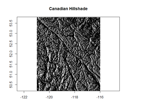
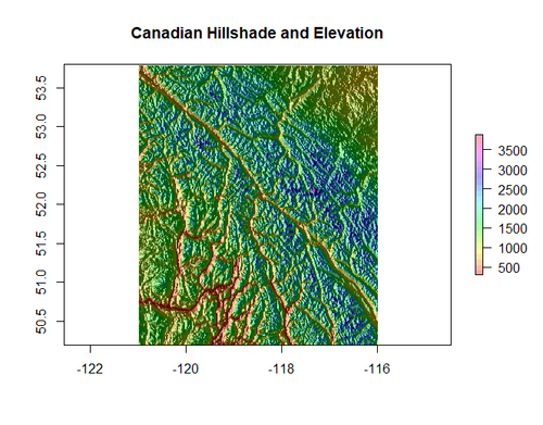
The hillshade function creates a 3D representation of the original DEM. This function is available within RStudio and is called gdalogr:hillshade. In order to use this function we will need to set the azimuth angle and slope, we will use 270 and 40 degrees respectively. Hillshade analysis is useful for generating 3D images representative of the DEM plot. First we will create a hillshade raster with the gdalogr:hillshade algorithm, then we will overlay the original DEM to provide elevation as additional context to the image.
#Hillshade function applied to the Canadian DEM, overlain by the original DEM
run_qgis(alg = "gdalogr:hillshade", INPUT = canada_dem_clip, AZIMUTH = 270,ALTITUDE=40,
         OUTPUT ='C://tutorial/canada_hillshadecan.tif')
canada_hillshade<-raster('C://tutorial/canada_hillshadecan.tif')
plot(canada_hillshade, col=grey(0:100/100), legend=FALSE, main='Canadian Hillshade and Elevation')
plot(canada_dem_clip, col=rainbow(25, alpha=0.35), add=TRUE)
Below you can see the output generated from the hillshade as well as the output generated by overlaying the DEM.
.
Conclusion
After finishing this tutorial my hope is that the user will have a functional workspace within RStudio in which they can utilize the various functions demonstrated. Additionally, I believe I have provided the tools necessary for users to explore and search for algorithms that they may need to use within their own projects. RStudio provides a unique environment for the user to create custom scripts to manage their geoprocessing algorithms.

