Extracting Shoreline Polygons and Polylines from Sentinel-2 Imagery

Introduction

The delineation of shoreline polygons can have a variety of practical applications from shipping and navigation to change detection and mapping coastal erosion. Often shoreline shapefiles are created using a semi-automated method combining automated boundary extraction and manual interpretation. This tutorial will focus on delineating shoreline polygons and polylines from Seninel-2 satellite data using the Naturalized Difference Water Index [NDWI] to define the boundary between water and land. This boundary will then be extracted and manually corrected to produce a final shoreline polygon and polyline file.

The purpose of this tutorial is to show the user how to extract shoreline polygons from satellite data in the Qgis software package. For this tutorial the Copernicus Open Access Hub will be used to access the required satellite imagery. The report will explore how to use this data portal to brows and download the available Sentinel-2 imagery. The satellite imagery will then be imported in to Qgis where polygons and polylines of the shoreline will be created.

Both Qgis and the Copernicus Open Access Hub are free to use, however the Copernicus Open Access Hub does require the user to create an account to download the data. The latest version of Qgis can be downloaded from the following link: (https://www.qgis.org/en/site/ )

Note: QGIS version 3.8.1. was used to create this tutorial. A newer version of the software may be available.

Data

This report will use Sentine-2 satellite data collected by the European Space Agency. The Copernicus Sentinel-2 satellite mission is a constellation of two multispectral polar orbiting satellites . The satellites offer data in the form of Level-1C and Level-2A data products. The Level-C1 products are multispectral satellite images that include the top of atmosphere reflectance. This means they do not have any atmospheric correction applied. Level-2A data products are derived from Level-1C data and offer bottom of atmosphere reflectance. In this case atmospheric corrections have been applied to the image to remove some effects of the atmosphere on the image’s reflectance . It is worth noting that Level-2A data may not be offered for many regions outside of Europe. For this reason, the study will use Level-1C data.

Both the Level-1C and Level-2A data products have differing spatial resolutions depending on the multispectral bands being viewed. This study will use the Red, Green, Blue and NIR bands. All four of these bands have a spatial resolution of 10m with a swath width of 290m. In addition, when the data is downloaded it is projected in the relevant UTM zone using the WGS 83 datum .

QGIS Methods and Instructions

Importing and Merging

Step 1.

• Open Qgis.
• Upload the .tif DTM images in QGIS by clicking on the Data Source Manager button . The Data Source Manager window will then appear.
• Select the folder where your files are saved, (this folder can be added to your favourites by right clicking the folder and adding it to your favourites) drag in all four .tif files to the main window (ignore the .tif.ovr files and only use the .tif files). Alternatively, you can double click each file separately to add them to the project one by one.
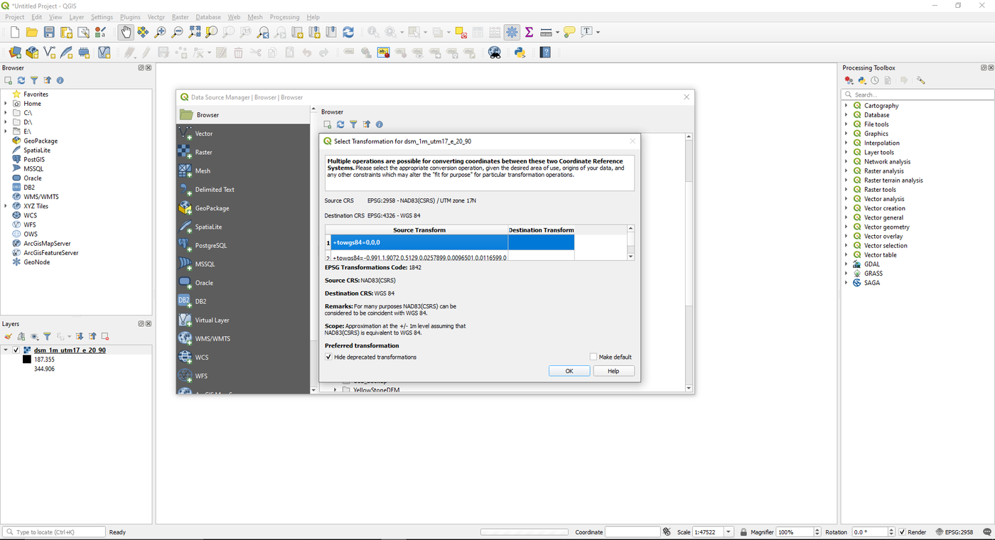
• A popup window will appear when you load in the .tif files, select the first option and click Ok.

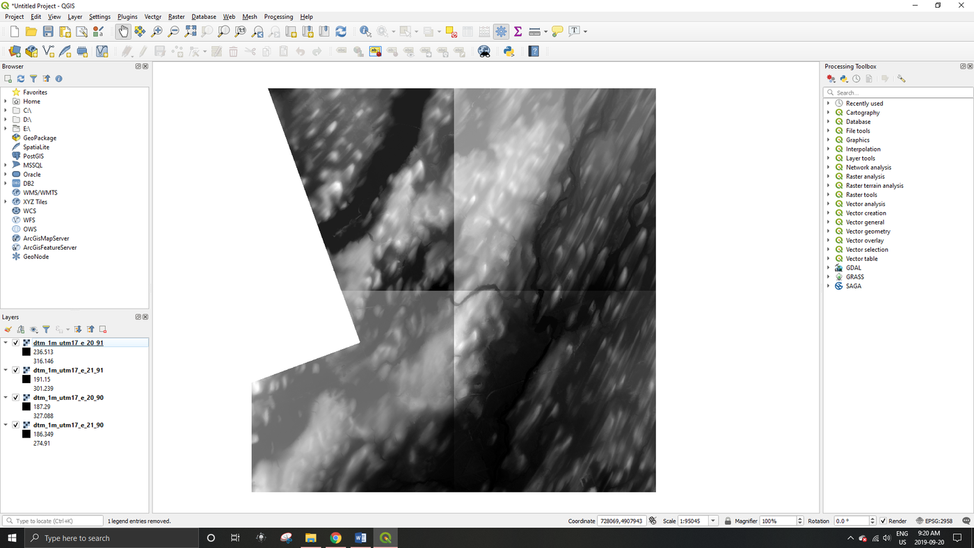
• The result should be the four raster images together in a square, as pictured below:
  • Note: If images are too hard to read, clicking on the image twice will result in a larger version of the image.