Vancouver-Whistler race planning with GRASS and QGIS
Introduction
The exceptionality about this project is to find a mountain bike route without on-site inspections of the terrain, roads or trails. The only data used for this project is of a digital nature and freely accessible on the web. The goal of this project is to create one of the hardest one day mountain bike-routes in the world. The approach is made through remote sensing of satellite images and digital topographic maps. With the aid of DEM (Digital Elevation Maps) a specific range of total altitude should be accomplished. The interval starts from 3500 meters in altitude to 6000 meters in altitude. Therefore several different routes should be found, in order to provide routes for every difficulty class. Hence the length of the route will vary. As the distance from Vancouver to Whistler on the Highway 1 is 126 km, it is likely that the distance for the different routes will range from at least 140 km to over 200 km. All the different routes will than be used for a mountain bike race, which will take place once a year in the summer, in which the different routes will represent different difficulties. Therefore it is possible that a wide range of people, from amateurs to professionals, from old to young, are able to accomplish the race. The data will be made accessible on the established race homepage, on the homepage of the Province of BC and on the website from BikeGIS in two different types of format:
- gpx format: GPS exchange format used to transfer data on any GPS
- kml format: for visualization on Google Earth, with background information, and pictures about the routes and surroundings
Working Process
In the following a detailed tutorial for all the important steps to realize this project is given.
Data Access
GIS Software
GIS Software captures, calculates, defines and visualizes spatial data. ESRI is one of the leading companys in selling their software ArcGIS. However there is also free available software on the net and two of them are GRASS and Quantum GIS. Download the most recent version of both software providers(GRASS 6.3 and Quantum GIS Version 0.11.0).
Data
For the actual data, we have to ask us the question, which kind of data is necessary to realize this project: Two things will be important
- a detailed map, with all the existing roads (from minor trails, over logging roads to major streets) to find a scenic but demanding route
- a digital elevation model to calculate the difference in altitude from the starting point and the finish. But also to calculate slope and indicate dangerous (steep) passages.
Both data can be found on two different internet sites:
- For DEM:
www.geobase.ca is a federal, provincial and territorial government initiative that is overseen by the Canadian Council on Geomatics (CCOG)
- For detaild maps:
www.GeoBC.ca download the required tif raster files (092g, 092j)
Working with Grass 6.3 & Quantum GIS
Both Software can be used for this project. However I used mor the Grass software for proeccising and analysing, and the Quantumg GIS software for visualization. Before you even open one of the Software, you should check the coordinate system of each data in the metadata:
- DEM
- topographic maps
In this case the projection system of DEM (NAD 1983) is different to the one of the topographic maps (NAD 1983 UTM 10N). This means that the data has to be reprojected, before it can be visualised on the same map. Open Grass 6.3. Two different Locations have to be created (DEM and TOPO). The easiest way is to click on the button "Georeferenced file", and choose one file from the downloaded data (for one Location one file from the DEM data, for the other Location one file from the topographic maps)
In the field "Project Location" two locations should be created now (DEM, topographic map). In each Location mapsets should be created in addition to the Permanent-Mapset (topo-Mapset, dem-Mapset). Import the raster files in each Mapset. It is always very important to adjust the Region extent with the g.region comand , because if the Region extent is too small for the layers, they won't appear in the Map Display window.
Reprojection
As we want to use the projection system NAD 1983 UTM 10 N (which is the projection for the topographic maps), the DEM data has to be reprojected to the TOPO-Location. For this process the topo-Mapset (and not the dem-Mapset!!!) has to be opened and with the command r.proj the DEM files can be importet to the TOPO-location.
Patch the Raster files
You probably realize that you now have a lot of raster files in your Location, which is not only unconvenient because you have to ad each raster file seperatly, which takes a lot of time, they also can't be used in later processes to calculate the elevation for the digitized mountain bike routes. r.patch is the command, where mutliple raster files can be united in one single raster ouput (use only those rasterfiles you really need for the analysis). However you have to make sure, that the region extent is set prior.
- dem_all
- topo_all
These two raster files is the only thing you need now for further analysis. It is also possible to patch the raster files, prior to the projection. This however didn't work in my case, probably due to the high amount of transfered data in one process.
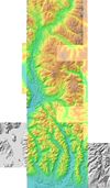
The visualization of both data could look like that:
Create Bike-Routes
Now it would be necessary to have a look at both maps (DEM, topo) to try to identify possible routes. Therefore look at areas (e.g. the valleys) without major routes, to see if there are minor roads, which can be used and which don't have a dead end. Take also a look on the web, and see if you can find even more detailed maps, such as hiking maps, which can be available in the different national- or provincial parks, located on the way. One example would be the Garibaldi-Provincial Park. These maps should be taken as a additional visual support in the process of digitization.
Digitization
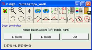
with the v.digit command, type
v.digit -n map=route 'bgcmd=d.rast map=topo_all'
in the Ouput window
-n means that you just created the vector with the name route. 'bgcmd=d.rast map=topo_all' means that wou will be able to see the map topo_all in the background, because that is the map you'll need to find the different routes. Even before you start to ditize you have to add a attribute table to the vector map, because otherwise the information you generate by digitizing can not be saved.
v.db.addtable map=route layer=1 'columns=cat integer'
The attribute table will be saved in your mapset under the directory dbf with the same name as the vector map (therefore route.dbf) and can be opened with Excel.
Now you can start to digitize:
- click on digitize new line
- the digit-tool window will get bigger and tells you in which layer (default=1) and in which category it will save the digitized line
- choose your digitized lines in that way, that on every cross section, where other potential routes can cross you start with a new category (see the green crosses on the map for digitized routes)
- after digitzigin click on the Save and Exit button
with the v.report command it is already possible to find out how long the different segments are:
v.report map=route option=length units=k
k stands for kilometres
Get Elevation data for the Routes
To find out how many meters of altitude each route will be, it is necessary to combine the route-vector map with the dem_all raster map. Therefore the vector map has to be changed from a line vector map to a point vector map.
With the command v.to.points points will be created along the line vector map:
v.to.points input=route output=points type=line llayer=1 dmax=100
The resulting points-vector map has to be sampled with the DEM-raster map:
v.sample input=points column=along output=points_z raster=dem_all
column=along is the column with the x,y coordinates. The name can be different, which can be checked by looking up the points.dbf file on excel, which was created automatically during the v.to.points process.
Calculating the altitude-profile in Excel
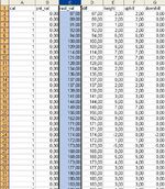
- Open the points_z.dbf file in excel
- all the points have four different columns:
- cat: gives you the number from which line this point originates
- pnt_val: changes with the change of the cat column
- rast_val: gives you the altidue of each point
- diff: is the difference between pnt-val and rast-val, but as pnt_val is not 0 all the time, the difference doesn't give the correct values for the elevation of each point
- three other colums have to be created
- Height: Difference between tow neighbouring points in altitude
- Uphill: gives you the positive value from one point to the next one and has to be calculated with the IF-Function, as negative values represent downhill values
- the formula should look like the following, where the E column is the Height Column, which was just created in the step before: =IF(E2<0;0;E2)
- Downhill: gives you the negative value from one point to the next one
- the formula is similar to the Uphill column and should look like that: =IF(E2>0;0;E2)
- Open Quantum GIS
- load the route vector map
- open the attribute table for the route vector map
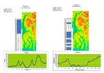
- select the rows, which will generate one route from Vancouve to Whistler (see table and the therefore selected lines on the map in the example route)
- Create new Excel files with the points, belonging to the selected Cat(egory) number in Quantum GIS
- therefore copy/paste the numbers in the new file (possible name: Route I, Route II, etc.)
- add a new column=distance in 100 m intervalls, as each point is approximately 100 m from the next one (see v.to.points the parameter dmax=100)
- plot the distance over the height to get the profile
- Sum up the downhill and the uphill values to get total downhill and total uphill
Export Data as KML files
KML format is used by Google Earth, which allows the user to visualise the different routes in Google Earth, even in 3D. The problem here is, that the files can't be exported in the TOPO-Location, as the chosen Coordinate System is not a geographic coordinate system (with degrees), which is used by Google Earth. Therefore the routes have to be reprojected to the DEM-Location, as this is a geographic coordinate system. This time the command is v.proj Open the dem-mapset under the DEM-Location and use the following command:
v.out.ogr in=route_1 dsn=route1.kml olayer=route_1 format=KML type=line
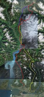
the files can now be visualised in Google Earth:
