Using QGIS to conduct watershed analysis and 3D modeling
Contents
Introduction and purpose
The purpose behind this tutorial is to show how QGIS can be used to conduct watershed analysis and how to create a 3D model of the Catchment area of the watershed using DEMs (Digital Elevation Model). This tutorial is meant to educate the user on how to conduct the analysis while introducing the theory behind it in a very simple manner in order for the user to understand the theory and apply the tutorial at the same time.
Acquiring DEMs
There are many websites that allow users to acquire DEMs, as a Carleton student, your best website you can use is the Geospatial Data Library of Carleton University linked HERE. Carleton University grants its student access to all sorts of geospatial data through its library and third parties like Scholars GeoPortal. For the purpose of this tutorial, I have found a DEM of rivers in Malaysia and will provide you with a link to the DEM if you would like to follow along. The link to the DEM can be downloaded from HERE.
Plug-ins installation
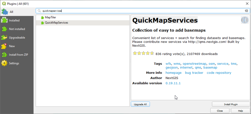
To help us reference the position of our DEM when we add it to our layers tab, the plug-in QuickMapServices will help us find easy and quick basemaps.
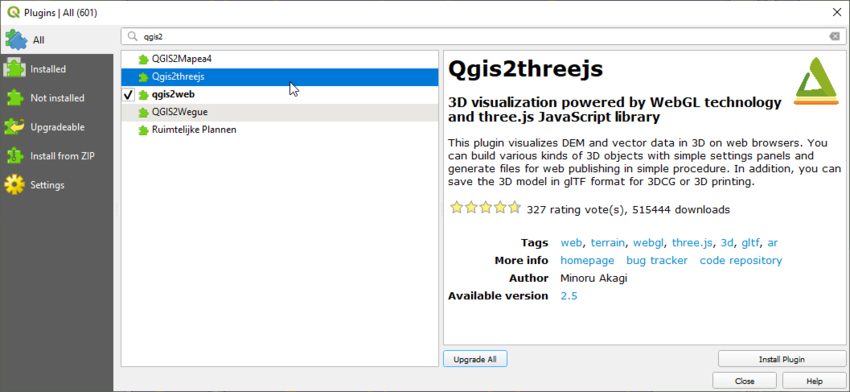
And to help us with 3D modeling, we will install the plug-in Qgis2threejs, which will use the elevation values in our DEM to create a 3D model of our catchment area.
Adding DEM and projecting
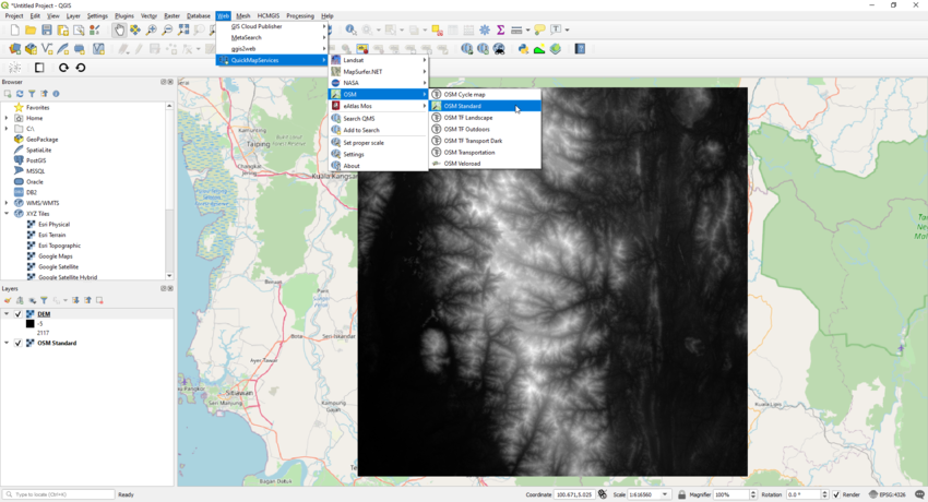
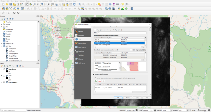
Once we add our DEM.tif file to our Layers, we use QuickMapServices to add a basemap. From our drop down menus, Web > QuickMapServices > OSM > OSM Standard. This will display Open Street Map in the backgound of our DEM as shown below:
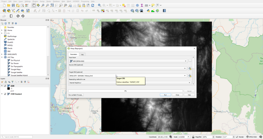
Next, we re-project our DEM to the appropriate projection, in our case -Malaysia- we can use GDM2000/Pahang Grid. Raster> Projections > Warp (Reproject) > Select GDM2000/Pahang Grid for target CRS. And from the bottom right hand corner, click on the projection icon, which will open the Project Properties, under CRS, chose GDM2000/Pahang Grid again.
After we are done with projections, the old DEM layer can be removed and we can rename the reporjected layer, for the sake of simplicity, it will be renamed Reprojected_DEM.
Now that we have our DEM ready, we can start the analysis!
Watershed Analysis
Step 1, Filling Sinks
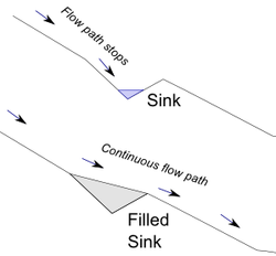
The very first step on our analysis is to what is called as Fill Sinks. The Fill Sinks tool by Wang & Liu produces a DEM free of depressions (AKA sinks) that would capture the flow of water, hence, conserving the waterflow in our data. The figure below is an example of a model with a "Sink" vs the same surface after filling the "Sink" and overland flow is continuous, which can be shown on Saga GIS tutorials website. [1]
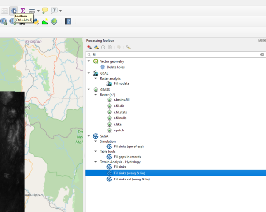
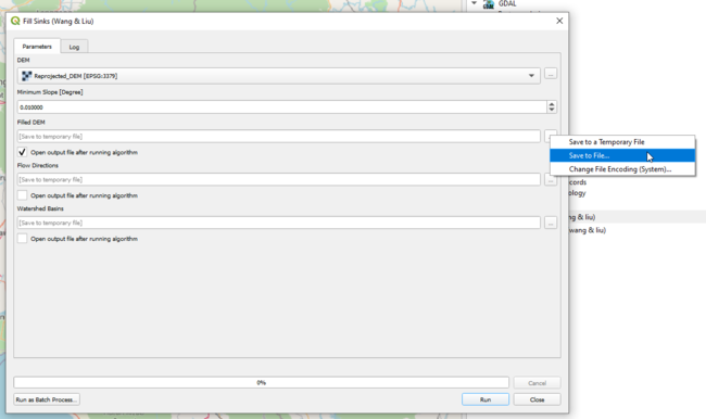
From Tools > SAGA > Fill sinks (wang & liu). Make sure to select the Reprojected_DEM and untick every option except (Open output file after running algorithm) and save to file using the 3 doted icon next to it. Hit RUN
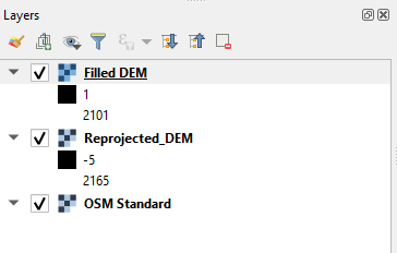
Notice the difference in our min and max values between the Filled DEM and our Reprojected_DEM:
Step 2, Strahler Order
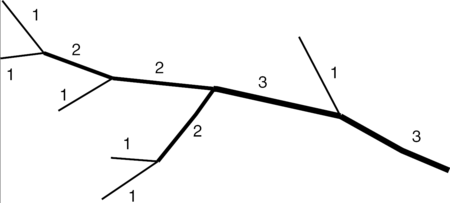
According to the system made by Strahler [2] [3], rivers of the first order are the outermost tributaries. If two streams of the same order meet, the resulting stream is given a number that is one higher. If two rivers of different stream orders meet, the resulting stream gets the higher of the two numbers. The following diagram showcases how Strahler Order works:
