Site suitability using SAGA GIS
Contents
Purpose
The purpose of this tutorial is to explain and show users how to perform a multi criterion analysis (MCE) on a dataset of their choosing using SAGA GIS. The example chosen in this tutorial is the production of a site suitability map to determine the best location for a windfarm in southern Manitoba.
Introduction
Wind energy refers to the process of creating electricity using the wind, or air flows that occur naturally in the earth's atmosphere. Modern wind turbines are used to capture kinetic energy from the wind and generate electricity. A collection of wind turbines is deemed a wind farm. Wind farms are best placed in locations that are near costal areas, or in open plains. Canada has 36 wind farms, with the majority being in Quebec and Ontario. What happens if we want to create a new wind farm somewhere? What are the factors we should be taking into consideration?
In this tutorial you will be given instructions to conduct a MCE in order to best determine the location of a wind farm in the region of Southern Manitoba bordering Saskatchewan.
Data
The data used in this tutorial is available through the Government of Manitoba's Land Initiative Website. The files used in this tutorial are a polygon shapefile of the Virden Region from 2006 and a shapefile of the City of Virden which includes buildings, utility lines, etc. To get ready for this tutorial, you should download all of these shapefiles and keep them in a working folder on your PC to make your work easier to locate.
Software required (SAGA GIS and QGIS)
System for Automated Geoscientific Analyses, also known as SAGA, is a great free and open source software package (FOSS GIS tool). It offers users a comprehensive and growing set of geoscientific methods and modules that allow for manipulating and analyzing vector or raster data. SAGA also allows for users to script in commands using its Command Line Interpreter (CMD). Despite being not very user friendly, the CMD has the advantage that it can be executed from batch script files, which in turn enables a further automation of complex work flows and the routine processing of mass data. QGIS is available for Windows and Linux.
Download the latest version of SAGA (v.7.9.0) to begin this tutorial.
Additionally, you should also have QGIS (v.3.14) installed as it is required in the very preliminary steps to make the data easier to work with.
Tutorial
Now that you have downloaded the software and shapefiles, it is time to begin.
Preparing the Data
Open QGIS and go to the Layer menu -> Add Layer -> Add Vector Layer. In the pop-up window, set your source type as File and click the Browse button under the Source header. Browse to where your shapefile is and double-click it or highlight it and select Open.
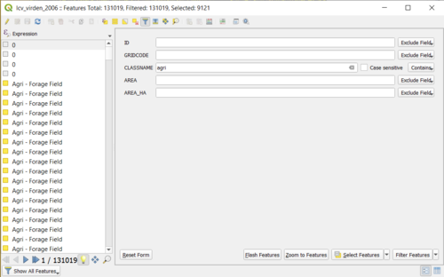
Upon opening the shapefile for the Virden region, proceed to right click the layer in the Layers window and click Open Attribute Table. Following this, click the Select/filter features using form button. On the far right of the window, beside the CLASSNAME field change the Excludes Field to Contains. Following this, in the field, type in agri and click the Select Features button at the bottom of the window. Doing so will highlight all the Agricultural and Agri - Forage Fields in the shapefile.
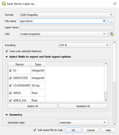
Close the attribute table and again right click the layer in the Layers window. This time click Export and select Save Selected Features As. This will open a new window. Enter the file name of your choosing and set the format to Esri Shapefile, then click OK. Doing so will create a new shapefile. In our case, it was called Agriculture.
Click the Deselect Features from All Layers button in the toolbar at the top, and then repeat the process again for all other classes in the original shapefile.
Adding Shapefiles into SAGA
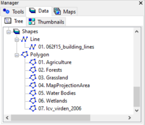
Launch SAGA and in the Data Sources window navigate to where your newly create shapefiles for all the different classes and the Virden City shapefiles are located. Clicking a file will automatically add it to the Manager Window under the Data tab. Do this for every shapefile.
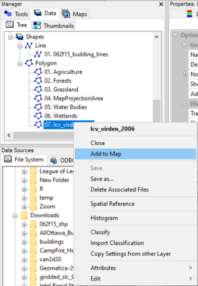
How SAGA works is that files can in the Data tab can be added to the Maps tab by simply right clicking the file and selecting Add to Map. If this is the first file you are doing this with, it will automatically create a new map with the name of the given file. For subsequent files, it will prompt you on which map you wish to add your chosen shapefile to.
Defining a Project Area and Creating Grid Maps
Grid maps are members of a specific grid system defined by a spatial extent and cell size. When a grid map is loaded into a SAGA work session, if the grid system it is a member did not already exist for the session, it is now listed along with any other loaded grid systems. In this tutorial, a specific grid system is defined for the project area and referred to as the project area grid system.
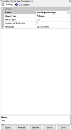
In order to define the project area first click the Tools tab, then click Shapes -> Tools -> Create New Shapes Layer. This will open a window as seen below
Enter the name you wish and change the Shape Type to Polygon, then hit Execute.
Once this new shape is created, add it to a map along with the other shapefiles we imported in the previous step. Note that because the shapefile has no actual shape to it, we must create one.
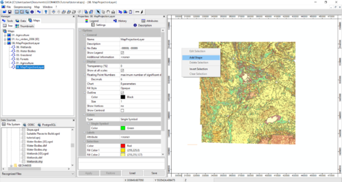
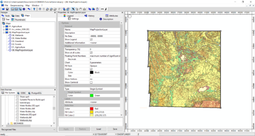
Begin by clicking the shapefile in the Map Tab, and then select the mouse button in the toolbar on the top of the screen (![]() ). Then click on the map itself to bring up a menu. Select Add Part and then begin to trace the outline of the completed shapefiles like below:
). Then click on the map itself to bring up a menu. Select Add Part and then begin to trace the outline of the completed shapefiles like below:
Once completed, the Layer will have a new instance, with the ID of 0. This will be used to create the grid system that will host the other grids we make in the next few steps.
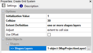
To create a new grid system, in the Tools tab, click Grid -> Tools -> Create Grid System. In the window that opens, change the Cell Size to 30, the Initialization Value to 1 and the Extent Definition to One or more shapes layers. In the >> Shapes Layers field, input the polygon that you created.
This will create a new grid definition with a value similar to: "30; 3647x 3868y; 321532.093525x 5427575.539568y"
When a new grid system is created, a dummy grid map is automatically created as a member of the new grid system.
Creating Constraints
The next step in the MCE, and something that is important to think about is where do we not want our wind farm to be located? Ideally it should be in a location that is far from civilization, is on dry land, away from forests and away from water bodies. This is what would be considered a constraint. In order to determine the best location for our future wind farm, we must create constraints for forested + urban areas and water bodies + wetlands.
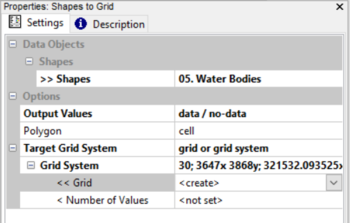
In order to build our constraint, we must first transform our shapefiles into grids by navigating to Grid -> Gridding -> Shapes to Grid and using the following settings:
- For >>Shapes input your desire shapefile (in our case it is our waterbodies shapefile)
- For Attribute select ID if it is not chosen.
- For Output Values select data/no-data.
- For Target Grid System select grid or grid system
- For Grid System select the grid system created in the Defining a Project Area and Creating Grid Maps step.
- Leave the <<Grid option as <create>
- Hit Execute
Repeat the above for the wetlands shapefile as well.
The above steps results in all water bodies and wetlands grid cells being assigned a value of 1 with all non-water grid cells that contain no-data being assigned a data value of 0.
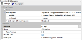
Once you have created your grids for both wetlands and water bodies, they must be combined into a single grid map. Navigate to Grid -> Calculus -> Grid Calculator and use the following settings:
- For >Grids enter the grids for both wetlands and water bodies
- For <<Result leave as <create>
- For Formula enter g1+g2
- Check the Use NoData box
- Hit Execute
- Right click the newly created grid and rename it to something of your liking
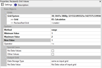
Upon creating this new grid map, it must be reclassified. Navigate to Grid -> Tools -> Reclassify Grid Values and use the following settings:
- For Method select range
- For Minimum Value input 1.0
- For Maximum Value input 2.0
- For New Value input 1.0
- For Operator select <=
- Deselect NoData Values and Other Values
- For  Data Storage Type select [same as input grid]
- For No Data Value under the Output Grid options, leave as No Data Value of Input Grid
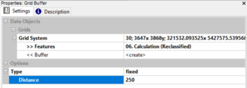
Once our grid has been reclassified, we must then create a buffer area around our new water gird features. To do this navigate to Grid -> Tools -> Grid Buffer and use the following settings:
- For >> Features choose your the reclassified grid you created in the previous step
- For << Buffer leave as <create>
- For Type select Fixed
- For Distance input a value of your choosing. The value chosen is presented in feet. Knowing this we chose a value of 250. If cell is to be chosen instead of fixed, then the value entered is the number of cells wide you wish for the buffer to be.
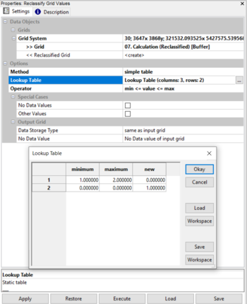
After creating our buffer, we must reclassify the grid once more to finally have our Water + Wetlands Constraint. Once again navigate to Grid -> Tools -> Reclassify Grid Values and use the following settings:
- For Method select Simple Table
   - In the Lookup Table that appears, use the following settings:
      - For Row 1, Minimum = 0.0, Maximum = 0.0, New = 1.0
      - For Row 2, Minimum = 1.0, Maximum = 2.0, New = 0.0
- For Operator select min <= value <= max
- Leave NoData Values and Other Values unchecked
- For  Data Storage Type select [same as input grid]
- For No Data Value under the Output Grid options, leave as No Data Value of Input Grid
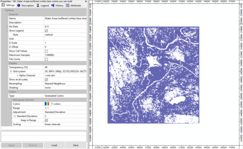
Once completed you should have something that looks similar to this:
As we can seen in the photo, all the areas that are in blue are areas that are outside the buffer range and can be considered areas that are viable for a windfarm.
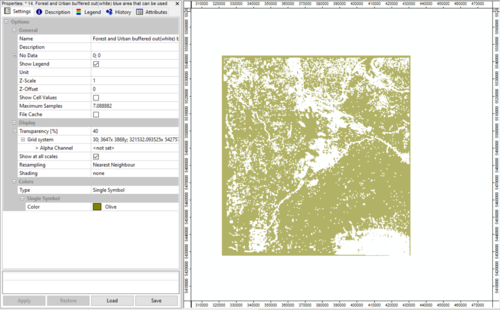
Repeat all the steps above for the Forests and Urban shapefiles to create a constraint for Forests and Urban areas. The result should look similar to below:
Using Boolean Aggregation to Create a Site Suitability Map
After we have created buffers for both the water + wetlands, and the forested + urban areas, we can proceed to creating our site suitability map. In this method, we will be using a Boolean aggregation approach, which is different from the weighted measures approach that is often seen in tools such as TerrSet software.
The Boolean aggregation approach takes all criteria from grid maps that contain 1s and 0s and allows them to be easily aggregated into a final solution using basic Boolean algebra. The tool that we will be using is the Grid Calculator which can be found by navigation to Grid -> Calculus -> Grid Calculator.
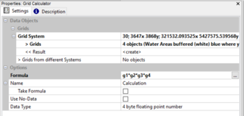
Once the tool is open, we must add in all of our constraint grids and all the areas we believe are suitable for the building of a wind farm, which in our case are the grasslands and the agricultural field grids we created at the beginning of the tutorial. Use the following settings to create the site suitability map:
- For > Grids choose your water + wetland constraint grid, your forested + urban constraint grid, your agricultural fields grid and your grassland grid.
- For << Result leave as <create>
- Leave > Grids from Different System as default
- For Formula enter g1*g2*g3*g4
- Enter a name of your choosing in the Name field
- Leave Take Formula and Use No-Data unchecked
- Set Data Type to 4 byte floating point number
- Hit Execute
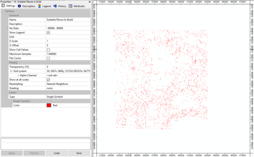
The result should be something similar to below:
Areas in red are the areas that are deemed to be suitable for building of a windfarm.
The output map has the value 1 where all areas of suitability intersect for all criteria and the value 0 for all areas that are unsuitable for one or more of the criteria. Suitability in one criterion cannot compensate for a lack of suitability in any other layer. They do not trade off. By meeting all criteria, the result is the best locations possible for the building of a wind farm.
Conclusion
SAGA when used with its GUI is a user-friendly software that provides users with many different tools and modules that aid in geoscientific analysis. In this tutorial SAGA was used to produce a site suitability map for the location of a wind farm in the Southern region of Manitoba bordering against Saskatchewan using the Boolean aggregation method. While straightforward, the method does not allow for any trade offs in the suitability of criterions. A weighted linear combination method is likely also possible to be completed using tools such as Fuzzify.
References
- Province of Manitoba. Manitoba Land Initiative | Core Maps - Data Warehouse | Digital Topographic Maps. Retrieved December 5, 2020, from Province of Manitoba: http://mli2.gov.mb.ca/t20k/topo062f.html
- Province of Manitoba. Manitoba Land Initiative | Core Maps - Data Warehouse | Land Use / Land Cover. Retrieved December 5, 2020, from Province of Manitoba: http://mli2.gov.mb.ca/landuse/index.html
- SAGA. Discover SAGA. Retrieved December 5, 2014, from SAGA: http://www.saga-gis.org/en/index.html
- SAGA. Download SAGA. Retrieved December 5, 2020, from QGIS: https://sourceforge.net/projects/saga-gis/files/SAGA%20-%207/
