Habitat Analysis using QGIS 3.22 and QuickMapServices Plugin
Contents
- 1 Purpose
- 2 Data Management and Setup
- 3 Data Management for the Tutorial
- 3.1 Organization of Shapefiles within your Computer
- 3.2 Setting up QGIS for Habitat Analysis
- 3.3 QGIS Coordinate Reference System Settings
- 3.4 Importing your Shapefiles
- 3.5 Creating Area of Interest and Clipping Shapefiles
- 3.6 Clipping Road Network and Water Network Shapefiles
- 3.7 Clipping DEM File by Mask
- 3.8 Saving your New Shapefiles and Updating Their Coordinate Reference Systems
- 4 Habitat Suitability Analysis
- 4.1 Habitat Restrictions
- 4.2 Restriction 1: Habitat must be located above 500m in elevation (Raster Calculator/Polygonize)
- 4.3 Turning Raster Data into Vector Data (Polygonize)
- 4.4 Elevation over 500m Results
- 4.5 Restriction 2: Habitat must be Located within 300m of a water source (Buffer and Fix Geometry)
- 4.6 Area within 300m of Water Results
- 4.7 Restriction 3: Habitat must be located at least 1 km away from any public road (Buffer and Fix Geometry)
- 4.8 Area's Located within 1km of a Roadway Results
- 5 Combining All of the Restriction Results
Purpose
The overall objective of this tutorial is to develop the spatial analysis and cartographic skills within the open-source software QGIS 3.22. By using the QuickMapServices plugin, users should be able to see the applicability of the add-on and be able to use it going forward in their own mapping careers. This tutorial will follow a step-by-step process that will determine ideal habitat locations for a hypothetical animal within Algonquin Park Ontario. With all of the data being open-sourced and QGIS being free, the entirety of this tutorial can be completed by anyone with a well-functioning computer or laptop.
Data Management and Setup
Required Programs and Plugins (Windows 64-Bit)
- The following programs are required to complete the tutorial. Please visit the URL’s attached and follow the steps to successfully install QGIS 3.22 (long-term release) along with the Open Layer Plugin. Please note: the following tutorial is being completed on a computer using Windows 10 as its OS.
Download Links
- 1) QGIS 3.22 [1]
Use of QuickMapServices Plugin
QuickMapServices plugin comes into play when developing final products. Their maps are often used as basemaps and they add additional spatial context to any project. In this case, we will be using the Google Satellite Imagery to display our data effectively. Please follow the guide below when installing the plugin and adding basemaps:
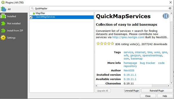
- Click on “Plugins” button located on the top menu of QGIS and select: “Manage and Install Plugins”. Search for “QuickMapServices” and install the plugin. Refer to the screenshot below if you run into any confusion:
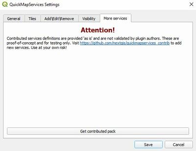
- Ensure the box is checked beside the plugin once it is completed installing. If this is checked, there will be additional menu items added to the top bar. From here, you can click on this new menu and begin to access the settings of this plugin. You can then access a “contributed pack” of basemaps that can be used in a variety of different situations. In this case, we will be using the Google Satellite basemap to add some additional context to our habitat analysis. Please refer to the screenshot below when trying to access these maps:
- These are the options available within the pack you have downloaded. As you can note by these pictures, there is a variety of different sources that supply basemaps. In most cases, you can use Google as a source because they supply a variety of different map types including satellite, road maps, and topographic maps. That being said, this pack should be considered as a staple within the library of any user of QGIS. These maps can be applied to almost any project as they add cartographic value to the end product.
- Please Note: These sources are constantly being updated therefore they are subjected to change. That being said, the majority of sources will remain constant unless they are being updated.
Using QuickMapServices within QGIS 3.22
By using completely open-sourced programs and data, this tutorial can be completed without any licensing issues. Open-source programs are often overlooked as they generally are claimed to be worse than their counterparts however this is not the case. Throughout this tutorial, you will be able to complete and visualize open source information effectively with the help of free plugins.
Data Management for the Tutorial
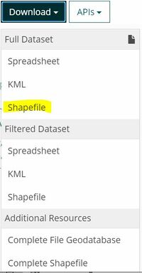
- Data being used are all accessible through Ontario GeoHub. When downloading the datasets, be sure to select the shapefile option within Ontario Geohub as this will be the format that we will be using later on in our tutorial. See image below for additional context.
- Download options available within Ontario GeoHub. These options can be accessed once a dataset is selected within the website and these options can be found on the right side of the website.
Organization of Shapefiles within your Computer
After you have downloaded all of the required files, it is strongly recommended to create a new folder within your C: drive that will act as a main directory for the project. This is very important as we will be dealing with a large number of shapefiles that will be changed in many different ways. This folder will also become the working directory and saving location for the project as a whole, therefore it will keep everything compact and easily accessible.
Setting up QGIS for Habitat Analysis
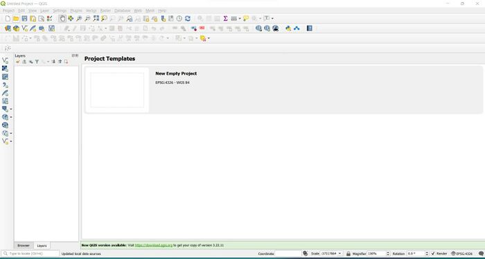
You can now open up QGIS for the first time as there will be an icon located on the desktop of your computer. You will be prompted by three different options within the middle of the screen and you will need to select “New Empty Project”. See below for a screenshot of this action.
- Screenshot indicating which option you are required to select when beginning a new project within QGIS 3.22. This option should always be selected when beginning any new task.
QGIS Coordinate Reference System Settings
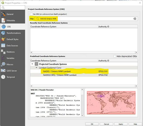
Prior to importing your shapefiles into QGIS, you are required to set a projected coordinate system for your new project file. In this case, all of the data being used was made accessible through the Ministry of Natural Resources, therefore we will be using their projected coordinate system known as “NAD83/ Ontario MNR Lambert”. This will ensure all of our analysis will be accurate and measured within useable units.
This menu can be accessed by the following path within the top menu of QGIS: Project -> Properties -> CRS. Specific projections can be searched by entering a projection known to work for a specific region in the "Filter" line. Should there be any question regarding the regional accuracy of the projection, a map view of the area covered is displayed for additional reference. Please see screenshot below for reference when setting up your CRS.
- This is what your CRS settings should look like prior to begging this project. It is crucial that you complete this step otherwise the data might become corrupt.
Importing your Shapefiles
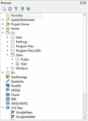
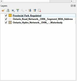
As mentioned above, now is the time you can import your shapefiles. You can import your shapefiles by using the browser menu within QGIS and located the folder within your C: drive (or wherever else you saved them). Select each shapefile, and drag it into the layers tab located underneath the browser tab. Your browser tab can be seen in the photo below and your imported shapefiles should be visible within the layers shapefile as seen in the image beneath.
Creating Area of Interest and Clipping Shapefiles
For practical use, we must begin clipping each shapefile as we are required to focus on a specific region within Ontario. For this tutorial we will be using Algonquin Park as our area of interest. Therefore, we must first select “Algonquin Park” from the “Provincial Park Regulated” shapefile and export the selected features. This will allow us to use this singular shapefile as the clipping method for the remaining three files (Road_Network, Hydro_Network and DEM). Please follow the steps listed below
- Toggle the “select by features or single click” tool within the top bar menu
- Click on Algonquin Park
- Right-click on Provincial Park Regulated Tab
- Click on Export -> Save Selected Feature As
- Save this file within your working directory and name it “AlgonquinBoundaries” and ensure the “add saved file to map” button is toggle on.
- You can now delete the original Provincial Park Regulated Shapefile and continue with AlgonquinBoundaries
Clipping Road Network and Water Network Shapefiles
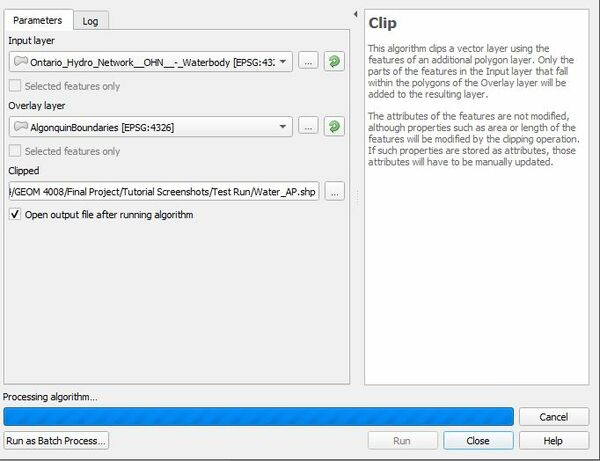
Moving forward, the “AlgonquinBoundaries” shapefile will be used as your reference file and you will begin clipping the other files to these extents. To do this please follow the instructions listed below:
- Under the “vector” tab within the top menu bar of QGIS, select these options: Vector -> Geoprocessing -> Clip.
- This will open up a clipping menu and you will need to use the following parameters:
- Run this algorithm and repeat the process for the road network shapefile as well (Substitute input layer for roads instead of water). This will result in two new layers being added to your document. Once these have both been completed, you can delete the original shapefiles titled “Ontario_Road_Network_ORN_Segment_With_Address” and “Ontario_Hydro_Network_OHN” as they will not be required moving forward.
Clipping DEM File by Mask
To clip a raster file, the process is similar however you must use a different tool within QGIS. To do this follow the steps below:
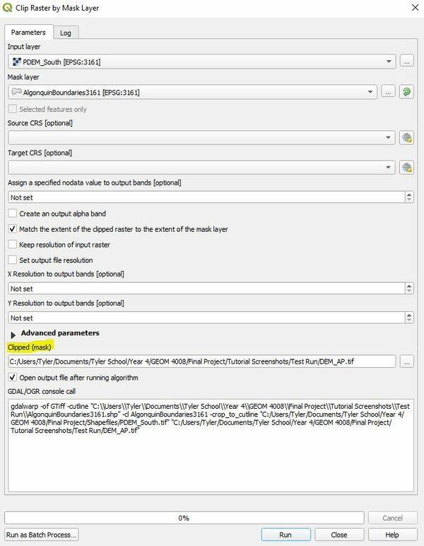
- Select “Raster -> Extraction -> Clip Raster by Mask Layer.
- Ensure you have the following parameters:
- You will now have all of your layers covering the extent of Algonquin Park and you are almost ready for analysis.
Saving your New Shapefiles and Updating Their Coordinate Reference Systems
Prior to doing any type of analysis we must ensure the shapefiles are using the same CRS as the project. To do this, you must follow the steps listed below:
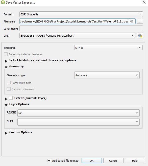
- Right click on a layer and select “Export -> Save Features As”
- This will result in a pop-up menu and ensure you have the following parameters set:
- You can now save the new shapefile and repeat the process with only the road network and hydro network shapefiles. You do not have to complete this process with the DEM file because it was already using this projected system when you downloaded it.
Habitat Suitability Analysis
Habitat Restrictions
For the purpose of this lab, we will be coming up with some habitat restrictions that will open the door for a variety of spatial analysis. Based on the open data collected, I have listed three hypothetical habitat restrictions below:
- Habitat must be located above 500m in elevation
- Habitat must be within 300m of a water source
- Habitat must be located at least 1 km away from any public road
To accommodate these restrictions, we must use a variety of different tools found throughout QGIS 3.
Restriction 1: Habitat must be located above 500m in elevation (Raster Calculator/Polygonize)
To accomplish this goal, we must use the raster calculator tool located within the top toolbar menu of QGIS. Please refer to the steps below when completing this process:
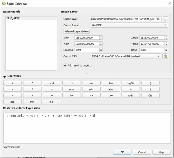
- Select these options from the top menu in QGIS: Raster -> Raster Calculator
- Use the following parameters:
- The new raster file will automatically be put into your layers tab and you can delete the older file.
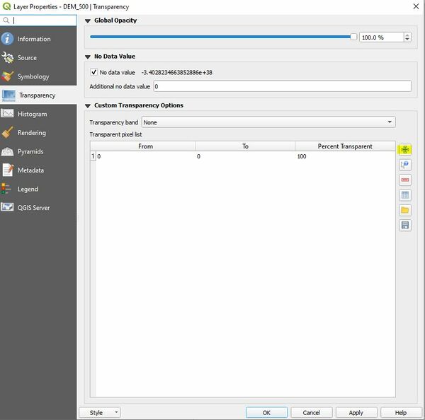
- To ensure this strategy will work, we must edit the transparency settings of this new raster file. This can be done by right clicking on the new layer and selecting Properties -> Transparency. Refer to the image below and ensure your document is similar. Be sure to set the “additional no value” to 0, then hit the highlighted “add” button to ensure we are following the same procedure.
- The overall purpose of this raster calculation is to divide the DEM file into areas that are located above 500m and below 500m. This not only limits the overall size of the file, it will allow for easier interpolation once we convert the file into vector format.
Turning Raster Data into Vector Data (Polygonize)
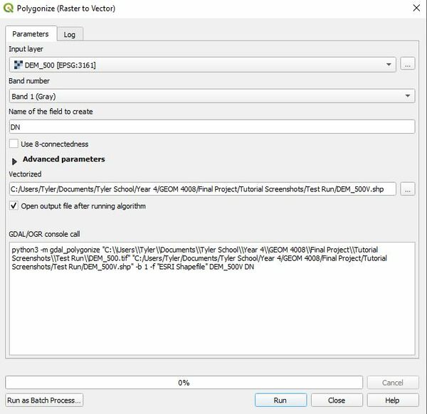
Prior to doing any relation analysis with the other shapefiles, we must convert this raster file into a vector polygon. To do this we must use the tool “Polygonize” which will help us convert easily. Please follow the steps listed below when converting the file:
- Click the following on the top menu of QGIS: “Raster -> Conversion -> Polygonize
- Ensure your settings resemble the following:
- From there, a new vector file will be created however it will all be the same colour. We are not interested in the area below 500m therefore we must manually edit the document to remove those locations from the shapefile. This can be accomplished by opening the attribute table and filtering the column “RN” by number and clicking the “edit button” within the top menu of the attribute table. From there, you can delete all of the values equal to 0 and this can be done efficiently by highlighting all of them and clicking the “delete button” within the attribute table. Once completed, save your edits and you should be left with a vector file displaying areas with high elevations.
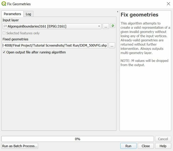
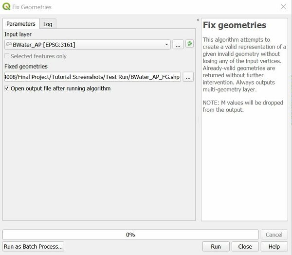
- Lastly, you must run the fix geometry tool on the shapefile as this will re-evaluate the accuracy of the new polygons and ensure there is no errors. This can be done by clicking on the “toolbox” icon within the top menu of QGIS and then searching for “fix geometries” within the toolbox menu. Ensure your settings resemble mine:
Elevation over 500m Results
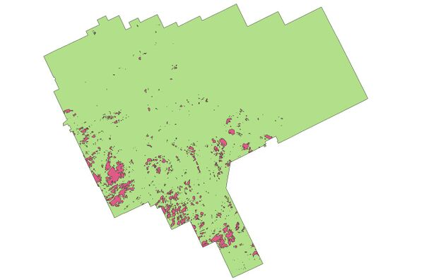
- This should be the result of the completion of each of the steps listed above. The pink areas are representative of areas that are above 500m in elevation and the areas below that mark are not included within the file. Therefore, the animal’s habitat we are looking to model must reside within the areas marked on the map below.
Restriction 2: Habitat must be Located within 300m of a water source (Buffer and Fix Geometry)
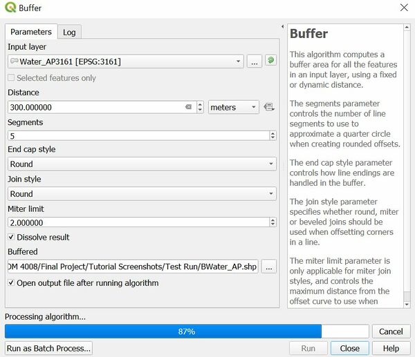
To accomplish this goal, we must create a 300m buffer around the waterbodies within the Algonquin area. This can be done easily following the steps provided below:
- From the top menu of QGIS select: Vector -> Geoprocessing Tools -> Buffer
- Ensure your buffer settings resemble the following:
- Run this algorithm. It can take some additional time because the hydro_network file is still relatively large even though it has been clipped.
- After this algorithm has run, you can now run the “fix geometries” tool within QGIS to validate the entire buffering process. This tool can be found by clicking the “toolbox” icon and then searching for it within the toolbox menu. Ensure your settings for the tool are the same as mine:
- This step is very important as it will help you avoid any errors when completing relational analysis between all three shapefiles later on in this tutorial. If you do not complete this step, the final buffers and clips will not work as there will be errors within the geometry of all the shapefiles you are using. Once you have completed all of these steps, you can delete the file named “BWater_AP” as we will be using the new shapefile named “BWater_AP_FG” moving forward.
Area within 300m of Water Results
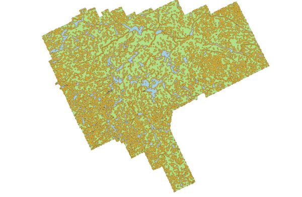
The result layer that was created will visualize 300m zones around any water source throughout Algonquin Park. With the hypothetical animal requiring a water-source near it’s habitat, it will reside in any area covered by yellow.
Restriction 3: Habitat must be located at least 1 km away from any public road (Buffer and Fix Geometry)
Yet again, we will be using the buffering tool accompanied by the fix geometry tool to achieve desired results. Please follow the steps listed below:
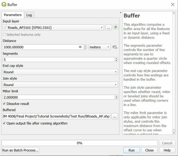
- From the top menu of QGIS select: Vector -> Geoprocessing Tools -> Buffer
- Ensure your buffer settings resemble the following:
- From there you can run the Fix Geometries tool with the same settings mentioned earlier in the tutorial. Please ensure you are giving the updated shapefile a new name and delete the older version when proceeding.
Area's Located within 1km of a Roadway Results
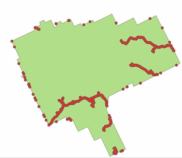
The results of your buffering and fix geometry process should resemble the following. All areas within 1km of a road will be marked in red therefore our hypothetical animal would not live within them.
Combining All of the Restriction Results
Clipping Buffered Water and Elevation Files
By completing a process like this, it will allow us to determine areas located above 500m in elevation that are situated within 300m of a water source. Please follow the steps below when completing the process:
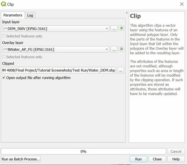
- Click on: Vector -> Geoprocessing Tools -> Clip
- Ensure you have the same settings as the screenshot below:
- The result will generate a map displaying areas that are suitable for the hypothetical animal however this does not encompass our last restriction which is roadways.
Difference Between Buffered Road Data and Combined Water/DEM Shapefile
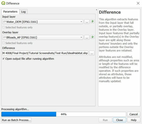
This is the last step in developing our hypothetical ideal habitat model. This step will allow the user to incorporate the last restriction on our results which will produce the final map. Please follow the instructions carefully as listed below:
- Click on: Vector -> Geoprocessing Tools -> Difference
- Use the same settings as I state below:
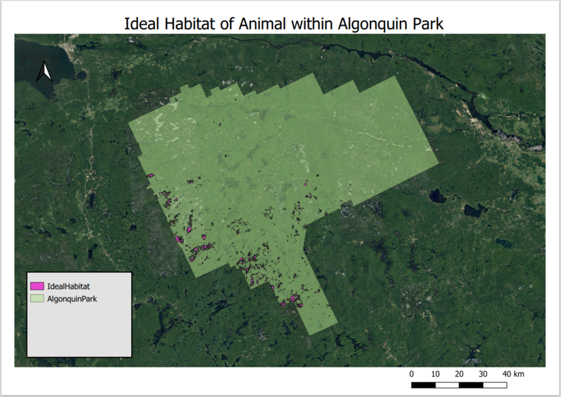
- Results should show the area that the animal could reside in while considering all three restrictions we have put on the land. New map layer should be created which should be named “IdealHabitat” as it will be your final product.

