Supervised and Unsupervised Image Classification with GRASS GIS
Hi all,
This tutorial will teach you how to perform supervised image classification in GrassGIS 8.4.0. This powerful open source software is renowned for its capabilities in handling geospatial data, making it a great tool for various applications like land use mapping, environmental monitoring and urban planning.
In this tutorial we will go through necessary steps to set up Grass GIS, prepare the data, create training areas and run a supervised classification.
Contents
- 1 Grass GIS Setup
- 2 Downloading Landsat Imagery
- 3 Creating a New Project
- 4 Importing Imagery
- 5 Mask Creation
- 6 Enhancing Bands
- 7 Creating a Natural Colour Composite Image
- 8 Defining the Study Area
- 9 Creating a group & subgroup
- 10 Supervised Classification
- 11 Unsupervised Classification
- 12 Generating an unsupervised classification
- 13 References
Grass GIS Setup
Grass GIS 8.4.0 (the latest version) can be downloaded at the following link. https://grass.osgeo.org/download/ Ensure to choose the correct version of Grass GIS for your operating system, whether that be MacOS, Windows or Linux.
Downloading Landsat Imagery
Landsat Imagery of Ottawa Ontario from November 2024 can be downloaded at the following link.
The data should then be put in an appropriately named folder on your computer that you can reference later in the tutorial.
Creating a New Project
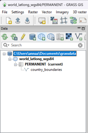
Once in Grass GIS, select the button that is a little globe with a green plus to create a new project location.
Give your project an appropriate name and an appropriate description. Hit next.
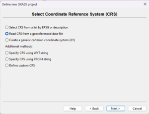
Under select coordinate reference system, choose “read CRS from a georeferenced data file." Then hit next.
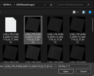
You will then be prompted to select a georeferenced file. Click browse. You will then navigate to the folder where you saved your Landsat imagery on your device. Within this file, we have a selection of imagery for each band from the particular date the imagery was collected. Each band is georeferenced to the same place, as they are all different versions of the same imagery. I selected band 1 (B1), although any band would be acceptable.
Click open. And then once the correct file is selected, hit next. This will set up the location of the project based on the geography of the imagery. You will then be promoted with a summary of the definition of your new grass project. Click finish.
Importing Imagery
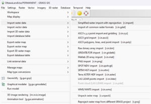
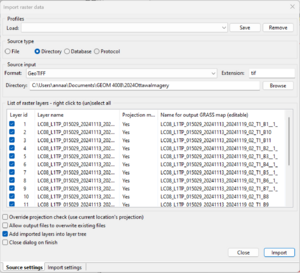
Next, we want to import our imagery of the Ottawa area. On the top ribbon, click file, then import raster data, then “simplified raster with reprojection.”
Select the directory under which you saved the Landsat data. Then under format, select GeoTIFF. This should make all of the associated Landsat files appear. Click import. Grab a coffee or a snack! This might take a little while.
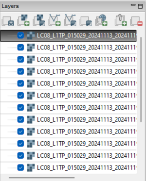
Once the images are finished importing, please close the import raster window. Under your “Bands” window, you have a “layers” window. This is where you can see all of the different spectral bands of the Landsat 8 imagery! Right now, the bands are all being displayed on top of one another, as all 11 of the boxes associated with each spectral band are selected.
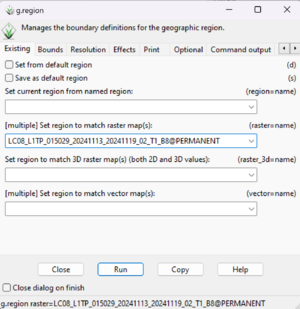
Next, we will set up a compilation area or a study area. One tile of Landsat 8 imagery covers quite a large area. Since we are only interested in classifying the Ottawa region, we will eliminate all unnecessary areas from our imagery. At the top ribbon, go to settings, set computational region, and set the region.
In the dialogue box that appears, we are going to set the computational region to match a raster map. The “raster maps” in question are the spectral bands associated with our imagery. Again, it doesn’t matter which band we use for this, as they are all georeferenced to the same location. In the 2nd box titled “set region to match raster maps” or “(raster=name)”, select the first band. Then hit run.
Once this command runs successfully, you can close the dialogue box.
Mask Creation
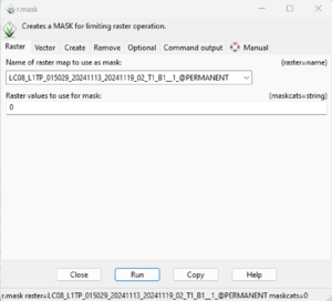
Next, we need to create a mask. Otherwise, the black background behind our selected Landsat swath will be classified with it. On the top ribbon, click raster, then click mask.
For the raster to use as the mask, select the 1st band again. Then enter 0 as the value to use for the mask. Then, at the top of the dialogue box ribbon, click the “Create” tab. Select “create inverse mask”. Then click run. When it is done running, close the window.
Enhancing Bands
At the top ribbon, click imagery, manage image colours and “colour balance for RGB”.
In the red box, select band 4 In the green box, select band 3 In the blue box, select band 2.
These are the bands we will use for our natural colour composite. This process will eliminate any unnecessary darkness in these raster layers.
Creating a Natural Colour Composite Image
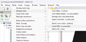
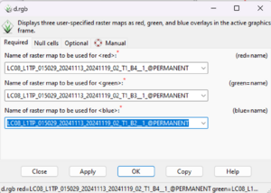
We must now create an RGB image using bands 4, 3, and 2 if our Landsat 8 imagery. At the top ribbon, click raster, then click manage colours, then “create RGB”.
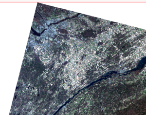
For the red band, use band 4; for the green band, use band 3 and for the blue band, use band 2. Then name your file something appropriate. I named my file “OttawaRGB432”; that way, I know exactly what bands are used in this image. Then select run. This will create another image in your layer tree. This band combination will show us what the Ottawa region looks like in natural colour, as it would appear to the naked eye from above.
Defining the Study Area
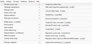
We are going to create a vector map. At the top ribbon, select vector. Then “develop vector map,” then “create new vector map.”
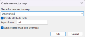
When you are asked to name the file, you can call it “OttawaArea” or something similar. Ensure that both boxes shown here are checked. Then press OK.
Press the magnifying glass with the plus signs beside it to zoom in to fit the entire image in your window.
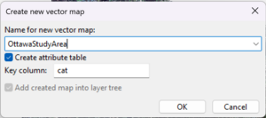
Then, on the “map display” ribbon, click where the “2D map” is currently displayed. Under that drop-down menu, select vector digitizer. Then, under the empty box’s drop-down menu, select “new vector map." Then give your new study area a name. I called mine “OttawaStudyArea.” Name it something memorable.
Pressing OK will cause an 'Attribute Table Manager' to appear. When this table pops up, simply close it. It has nothing to do with what we are trying to accomplish here. Take note of how 'OttawaStudyArea' is now in our layer tree!
Now go to your display layer and zoom into the area that you would like to analyze. For the purposes of this project, we will be focusing on the top right corner of the raster layer, which is where the city of Ottawa is located.
Then, within the map display window, select “digitize new area.”.
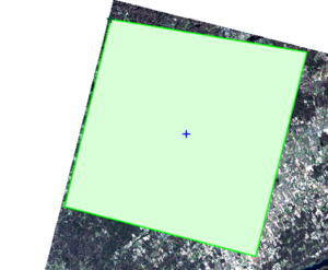
From there, define the boundaries of your study area. This does not have to be perfect; it simply has to encapsulate the area you wish to classify. Right-click to end the line.
You will be met with another dialogue box labelled “define attributes." Click submit. You can exit the digitization window using the power off button in the map display window. When you are prompted to save changes, click yes.
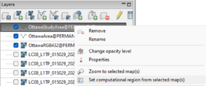
In your layer tree, right-click “Ottawastudyarea”, and select “set computation region from selected maps.”
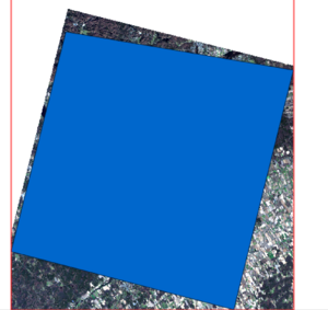
If your polygon has turned a solid colour, it means your study area has been successfully defined!
Creating a group & subgroup
We will need to create a layer group in which we will complete our analysis.
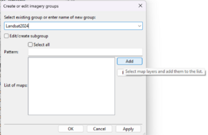
Under the main top ribbon, click imagery, then “Develop images and groups,” then “Create / edit groups [igroups].”
Create an appropriate name for the group. Then click add so that we can add each layer we can use in the analysis. For us, these will be bands 1 through 7. 8 and 9 are panchromatic, and above are thermal infrared, which we will not be making use of in this tutorial. Then, create a subgroup, and call it Ottawa2024. Within the subgroup, select all of the bands available (which are bands 1 through 7). Click OK. Now we have a group and a subgroup!
Supervised Classification
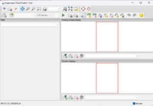
On the top ribbon, go to imagery, select classify, and then select interactive input for supervised classification. This will open up the classification window.
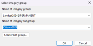
The first thing we do is select the group and subgroup we just made in the previous step! This is done with the paper and paperclip icon in the corner of the window.
The group and subgroup are now set up for this classification. Now we need an image to classify. Now, we will add the 3 same bands we used to create our study area image into our classification window. In the training area display, select ‘Add RGB map layer’.
Just as we created the RGB image in the above steps, we will select bands 4, 3, and 2 for bands red, green, and blue, respectively.
Click zoom to select map layers to have the image displayed in the clipped area we designated earlier.
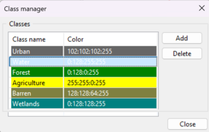
Select the class manager.
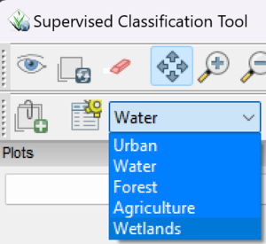
Now it's time to start training the image! The class that I will begin with is the water class. Within the training window, select the drop-down menu and select the water class.
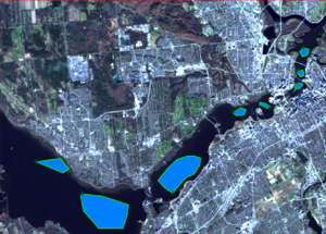
Zoom in on the areas of the image where you will create your training areas. Then click ‘Digitize new boundary area’.
You can then begin to create polygons in which all pixel values within the polygons represent water reflectance values. You should try to create multiple polygons each covering a small area with varying values of reflectance of the surface at hand.
Once you are happy with your training areas, you can move on to your next class. This can be accomplished by simply selecting the drop-down menu next to the class manager and clicking on the class you want to create training areas for next. Repeat this step for each of the classes.
Now it's time to save the polygons as a vector layer!
At the top of the digitization window there is a button that will allow you to export your training areas to a vector map. Click this button.
You will also be prompted to enter a name for the vector map. Name it something memorable and click OK.
You can then close your classification tool. We will then need to convert those vectors to raster and add them to our tree of layers. At the top ribbon, click vector, then map type conversion, then vector to raster.
For the input map, select your training polygon vector file. Then assign an appropriate name for the output raster. The source of the raster values will be ‘attr’. Then in the attributes tab, change the ‘att’ parameter to ‘cat,’ and the ‘name of the column used for raster category labels’ should be changed to ‘class.’ Then hit run.
As you can see, our training areas are now in our study area, and the new raster file containing our training areas is in our layer tree.
Now we are finally going to create a map from our training areas.
Under imagery at the top ribbon, select classify an image, and then “input for supervised MLC.” For ground truth training, you will select the raster you created in the last step. For the input imagery group, you will select the group you created in the previous step, containing the bands 1 through 7. The subgroup will be the same subgroup, with bands 1 through 7. Please name the output file appropriately to match the results of your classification. Then hit run. You now have a file containing the results of your classification. At the top ribbon under imagery, go to classify image again. This time, select maximum likelihood classification.
This will create another raster in your layer tree with the results of your classification. Congratulations! Take a close look at your map. Do the colours represent the land underneath? Where do you feel your classification is the most accurate? Where do you feel it is the least accurate? What did my training areas look like in this place? Were they large or small? Numerous or few? Spaced out, or close together? These are all questions you can ask yourself to gain a better understanding of how you can produce an even better classification in the future.
Your classification might not look perfect on the first go – and that’s totally okay. Classifications rarely are. The purpose of this tutorial was to help you gain an understanding of how to do supervised classifications in Grass GIS. If you were ever asked to do the classification of satellite imagery at a professional level, it could take weeks or even months!
Unsupervised Classification
With supervised classification, we allow our computers to do the majority of the heavy classification lifting for us. GrassGIS will automatically pick out classes of band frequencies within the image. The user's job is to identify the correct number of classes for your image and to define what these classes represent. Unsupervised classifications are an iterative process, meaning that different results will be produced whenever the maximum likelihood classification is run. This is necessary, as the first classification created by the computer may not necessarily be the best. Your results may be different than the ones produced in this tutorial, and that is to be expected.
Creating a cluster
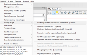
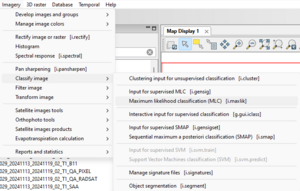
At the top ribbon, select the imagery tab. Under "classify image", choose "clustering input for unsupervised classification".
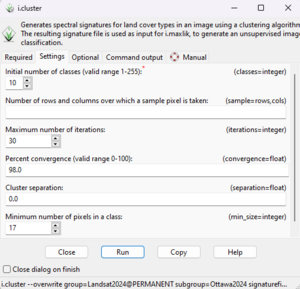
The name of the Input Imagery group will be the same as the one we created in the supervised classification tutorial. The name of the imagery subgroup will again be the same as the one we created previously. Choose an appropriate name for the output file.
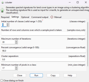
Under the settings tab in the i.cluster window, select the appropriate amount of classes that the clustering algorithm should create. The number of classes, like in the supervised classification tutorial, should reflect the amount of different land uses you believe to exist within the imagery. For the purposes of this tutorial, I selected 6. You can leave the rest of the setting as default.
Under "Optional", select "allow output files to overwrite existing files". This box should be selected, as you will likely need to repeat this process several times until you are met with an output you are happy with, which will be different from user to user. Checking this box allows the newest output to overwrite and delete the last output. If ever the user wanted to keep both the previous output and create new ones, this box could be unchecked.
Hit run.
Generating an unsupervised classification
Once this step is completed, at the top ribbon under "imagery" selec the "classify image" option, then select "maximum likelihood classification". This step will create a computer generated classification scheme.
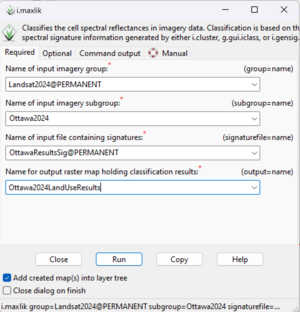
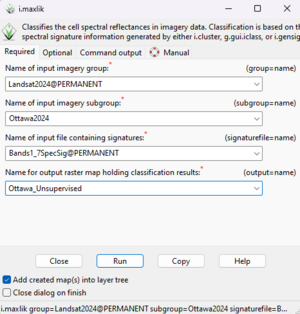
Once in the "i.maxlik" window, select your already made imagery group as the input imagery group, as well as your imagery subgroup as the input subgroup. Then select the file created in the previous step as the name of your input file containing the spectral signatures. Create an appropriate name for the output of the maximum likelihood classification.
Then click run.
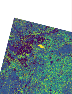
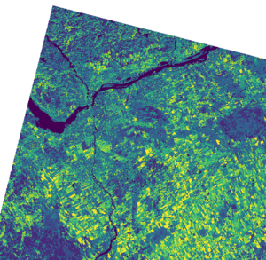
The resulting classification will then be displayed in a default colour scheme.
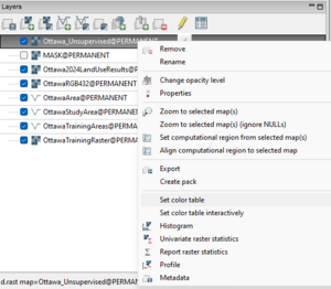
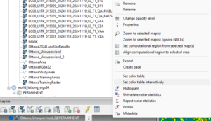
In order to gain a better understanding of the classification created by the computer, the colour scheme should be changed. In the "layers" pane, right click the supervised classification output layer that is currently being displayed on your screen. Select "Set colour table".
In the "define" tab of the r.colours window, set the "name of colour window" to "random".
With this selected, each class generated by the GrassGIS will be displayed in a unique random colour.
Now that the classes generated with supervised classification can be clearly distinguished, you may or may not be happy with the result. If you are unhappy with the result of this classification, feel free to return to the "creating a cluster" step again. Under the settings tab of this window, the user can adjust each of the settings beyond their default value as they see fit.
Once the user has an output they are happy with, they can move on to the final step, which is assigning a real world purpose to each of the classes generated by the computer.
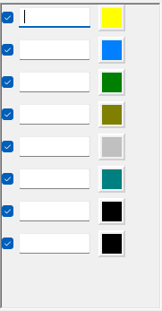
To do this, under the layers tab once again, right click the output layer generated by the cimpuert that is displayed on your screen. This time, select "set colour table interactively".
You can now assign an appropriate colour to each class in your imagery. For the purposes of this tutorial, I chose the same colours as in the unsupervised classification, but you can choose whatever works best for your image.
Conclusion
This brings us to the end of our tutorial! I hope this helped you learn about classifying images in Grass GIS.
References
GRASS Development Team. “I.Cluster.” I.Cluster - Grass Gis Manual, grass.osgeo.org/grass-stable/manuals/i.cluster.html#:~:text=This%20parameter%20determines%20the%20maximum,may%20want%20to%20rerun%20i.
GRASS Development Team. “Classifying Images.” Classifying Images, grass.osgeo.org/gdp/grass5tutor/HTML_en/c1622.html.
GRASS Development Team. “I.Group.” I.Group - Grass Gis Manual, grass.osgeo.org/grass-stable/manuals/i.group.html.
GRASS Development Team. “I.Maxlik.” I.Maxlik - Grass Gis Manual, grass.osgeo.org/grass-stable/manuals/i.maxlik.html.
GRASS Development Team. “I.Class.” Grass GIS Manual: I.Class, grass.osgeo.org/grass65/manuals/i.class.html.
GRASS Development Team. “Topic: Classification.” Grass GIS 8.5.0dev Reference Manual: Topic Classification - Grass Gis Manual, grass.osgeo.org/grass-devel/manuals/topic_classification.html.
